Engineering
Building a Causal Attribution Engine for AI-Powered Root Cause Analysis
By Pratham Bhonge, Bharath Harish
A monitoring alert can tell you, “Daily Revenue dropped 18%.” You know what happened, but you don’t know why it happened.
Traditional dashboards give you breakdowns, like revenue by region, channel, and product. But breakdowns alone can’t distinguish correlation from causation. They can't tell you whether the drop in the West region caused the revenue decline, or whether both were symptoms of a deeper issue, like an ad spend cutback three days earlier.
That gap is where a causal attribution engine becomes useful. This article focuses on the statistical attribution engine: it decomposes metric anomalies into structural signals, anomaly attribution scores, and causal chains. Those outputs are then consumed by an AI incident-investigation agent, which verifies each hypothesis with SQL, explores related dimensions, and writes the final human-readable RCA. Three questions are answered in order — Where did the delta come from? Which drivers caused it? What end-to-end story best explains it? This layered design is important because every eventual decision depends on the graph and scoring choices made up front.
Layer | Question | Method |
|---|---|---|
Structural (WHERE) | Which sub-components explain the delta? | Compositional decomposition |
Causal (WHY) | Which drivers caused the change? | Toda-Yamamoto Granger causality + Pearson correlation |
Narrative (THE STORY) | What's the end-to-end root cause chain? | Path tracing through causal + structural edges |
The output feeds directly into an AI agent that verifies each hypothesis with SQL, cross-references dimensions, and produces a human-readable incident report.
What The Workspace Graph Looks Like
Before attribution runs, there must exist a directed acyclic graph connecting metrics. This is the workspace graph.
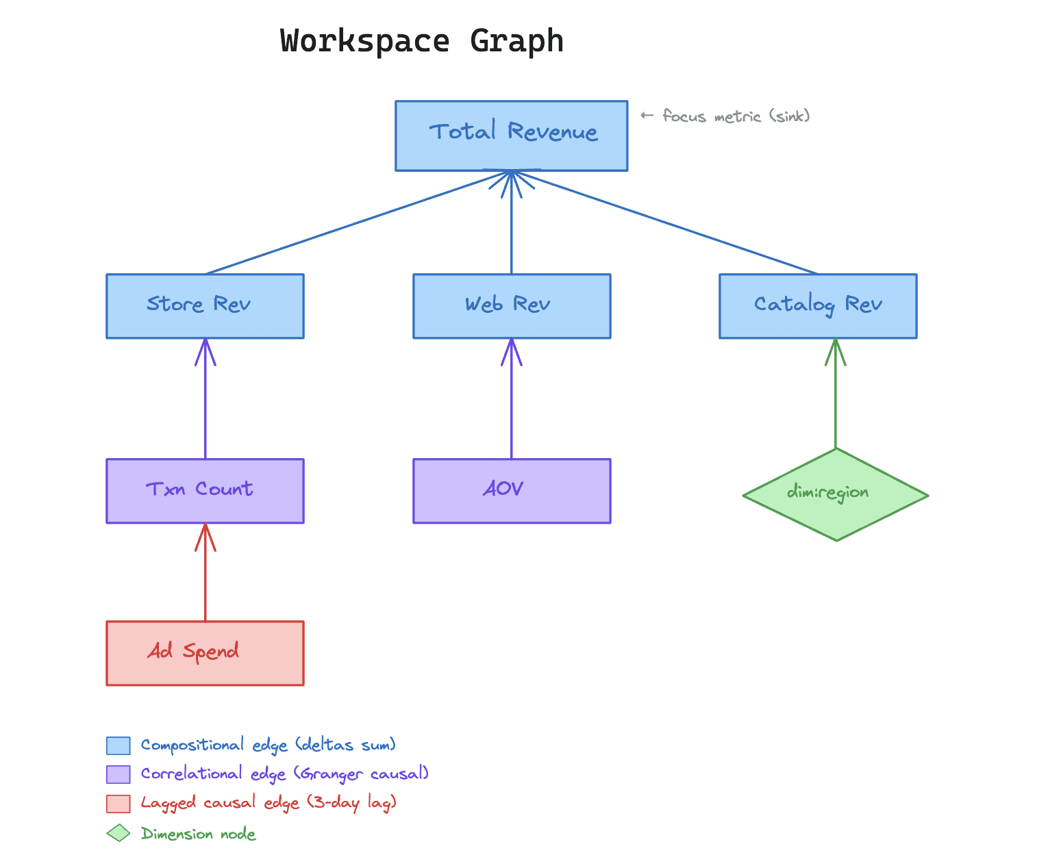
Nodes are metrics (UUIDs) or dimensions (dimension:region)
Edges are directional — source drives target:
Compositional edges: Store Rev + Web Rev + Catalog Rev = Total Revenue
Correlational edges: Ad Spend → Txn Count (causal, possibly lagged)
At build time, all edges have weight = 0. Weights are computed live during attribution, so there are no stale pre-computed scores. Once that workspace graph exists, the pipeline can move from time-series fetch to ranked explanation.
The Attribution Pipeline
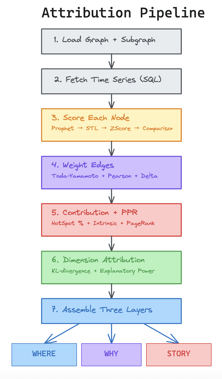
The entry point is run_full_attribution(). The 16-step flow can be read as seven larger stages. The graph and the relevant subgraph are loaded. Time series are fetched with SQL. Each node is scored for current anomaly strength. Edges are weighted with Toda-Yamamoto Granger causality, Pearson amplification, and delta alignment. Contribution and Personalized PageRank are computed. Dimension attribution is run. Finally, the output is assembled into WHERE, WHY, and STORY layers. That ordering is not cosmetic. Statistical choices made early, especially metric typing and series transforms, decide whether the causal layer will be trustworthy.
Type-Aware Recipes
Not all metrics are the same. For example, a ratio metric (Conversion Rate = Orders/Sessions) can't be decomposed the same way as an additive metric (Revenue = Σ order amounts). We classify each metric into one of 10 types and assign a recipe that controls scorer choice, transform choice, edge decomposition, dimension slicing, and drill guidance. This design keeps the engine auditable instead of turning it into a pile of ‘per-metric exceptions.’
Metric Type | Transform | Decomposer | Why |
|---|---|---|---|
Additive (Revenue, Count) | diff | Additive | First-difference removes trend; deltas sum exactly |
Ratio (AOV, CTR) | log_diff | Ratio (Taylor) | Log maps R+ to R, diff removes unit root |
Proportion (Channel Share) | clr | Simplex | Centered log-ratio for compositional data on the simplex |
Cumulative (QTD Revenue) | rate_of_change | Pace | Level comparison is meaningless; pace is what matters |
Snapshot (Inventory Level) | none | Structural | Point-in-time; no differencing needed |
This recipe system is one of the most differentiated parts of the engine. Raw ratios can produce spurious results because the series do not live in an additive space; per-type transforms are therefore applied before VAR fitting. Once the metric space has been normalized, anomaly scoring becomes much more reliable.
Metric Anomaly Detection and Scoring
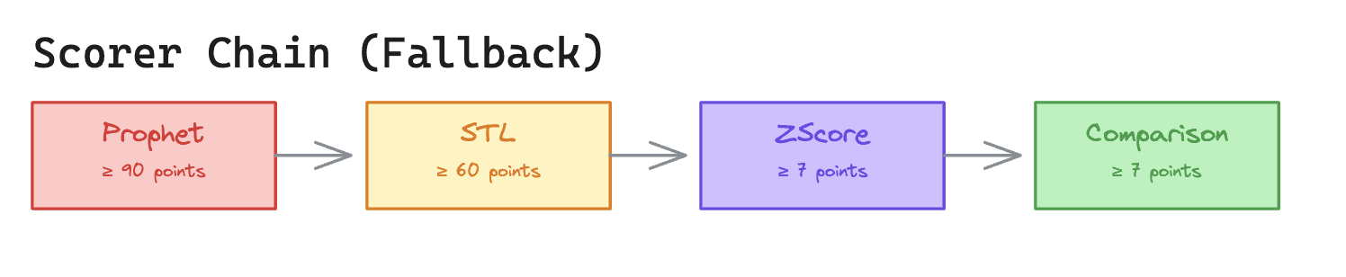
Each metric node is scored for how anomalous it is right now through a scorer chain. The order is deliberate. A richer model is tried first, and a simpler model is used only when the data history is too short.
Scorer | Min Points | Method | Fallback Behavior |
|---|---|---|---|
Prophet | 90 | Facebook Prophet forecast interval | → STL |
STL | 60 | Seasonal-Trend decomposition, score residual | → ZScore |
ZScore | 7 | z = (value - μ) / σ over trailing 30d window | → Comparison |
Comparison | 7 | Week-over-week % change | terminal fallback |
Regime Detection
We run CUSUM changepoint detection on the baseline period before scoring. If a structural shift above 20% is detected, only post-shift values are used. This prevents a regime change (e.g., a December seasonal ramp) from inflating anomaly scores.
This is validated in our stress tests: Scenario L (Seasonal Ramp + Drop) and Scenario M (Regime Change + Dip) specifically test this. Once anomaly scores are stable, we shift our focus from what moved to what drove the move.
Edge Weighting With Toda-Yamamoto Granger Causality
This is where the statistical load is carried. For every edge, we compute structural and causal weights. Structural weight starts with simple delta decomposition:
For ratio metrics, we use a Taylor expansion: δR ≈ (1/D₀)·δN − (N₀/D₀²)·δD, correctly attributing ratio changes to numerator vs denominator.
But, why Toda-Yamamoto?
The causal side is where Toda-Yamamoto Granger causality matters. Standard Granger causality usually requires stationary series, so pre-differencing is often forced. That can remove level information and introduce extra model-selection uncertainty. Toda and Yamamoto sidestep that by fitting VAR(p + d_max), then testing only the first p lags. Here are the method steps:
Fit VAR(p + d_max) where p is AIC-selected lag order and d_max = 1 (integration order buffer)
Run a Wald test on only the first p lags
The extra d_max lags absorb non-stationarity without requiring pre-differencing
The final causal strength is a combination of Granger output, Pearson alignment, anomaly strength, and direction consistency:
A key design choice is the binary direction_alignment term. If the source moved opposite to the focus delta, causal weight is forced to zero. A metric that increased while revenue decreased is not accepted as the driver of the decrease. At this stage, anomaly attribution stops being a correlation-only ranking and becomes a constrained causal estimate.
Contribution and Dimension Attribution
Once edge weights have been set, two complementary node scores are produced. contribution_pct measures how much of the focus delta is explained by a node, while intrinsic_score estimates how much of a node’s movement remains unexplained by its parents. We need both node scores: one for scale-normalized contribution and the other for root-cause novelty.
HotSpot Contribution (contribution_pct)
“Store Revenue explains 72% of Total Revenue's change.” It's simple, interpretable, and scale-normalized.
Intrinsic Anomaly Score (DoWhy ICC approximation)
But, how much of a node's movement is unexplained by its parents? This is the key to root cause identification
Leaf nodes = no parents. Therefore, all movement is intrinsic (intrinsic = anomaly_score)
Intermediate nodes that moved exactly as predicted by parents collapse toward zero intrinsic score
Nodes with intrinsic > 0.3 are flagged as root cause candidates
Personalized PageRank
A backward Personalized PageRank pass is then added so blame can be distributed through the graph rather than being pinned only to immediate parents.
The final ranking formula will now look like this:
Dimension Attribution
Dimension attribution follows an Adtributor-style design. The design measures surprise with KL divergence on share shifts, and measures explanatory power by slice_delta / |total_delta|. The impact score is the result of suprise and explanatory power.
We normalize to daily averages before computing shares, making the comparison period-length-independent, meaning we can compare a 7-day anomaly window with a 14-day baseline without period-length bias.
The impact_score returns top-k slices: five by default. At this point, structural contribution, anomaly attribution, and dimension attribution are ready to be merged into an output that the agent can act on.
The Three Output Layers
The merge we spoke about in the previous section is exposed through three output layers instead of one monolithic ranking.
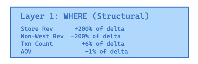
Layer 1: Structural Breakdown (WHERE)
This layer answers ‘WHERE’ by walking compositional edges backward from the focus metric and reporting contribution percentages.
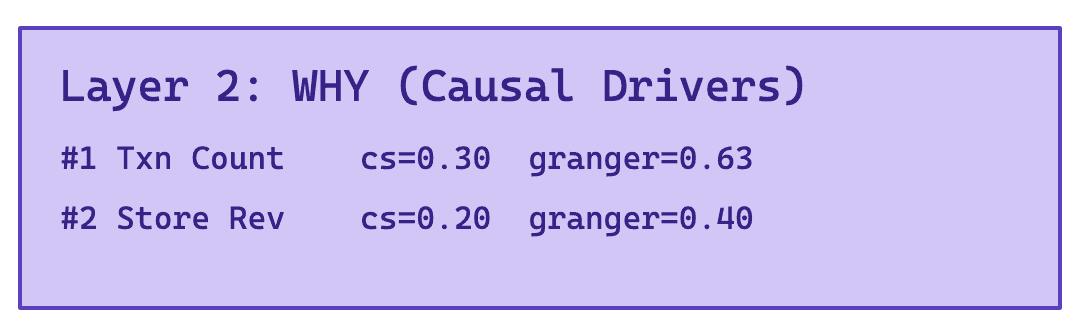
Layer 2: Causal Drivers (WHY)
This layer answers ‘WHY’ by ranking edges with causal_strength > 0.01.
Layer 3: Causal Chains (THE STORY)
This layer answers ‘THE STORY’ by stitching causal and structural edges into end-to-end narratives.
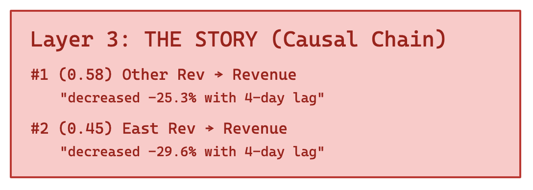
chain_score = causal_strength × |contribution_pct of driven branch|
This split is what makes the system usable in AI-powered root cause analysis. ‘WHERE’ tells the agent which branch should be inspected first. ‘WHY’ highlights the most likely causal drivers. ‘THE STORY’ turns those signals into causal chains that can be verified in order rather than being guessed from scratch.
How the Agent Uses Attribution
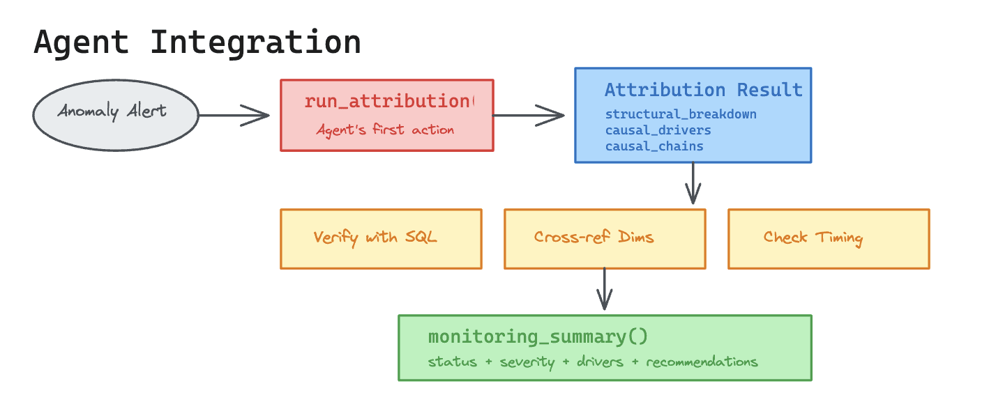
In practice, run_attribution() is called as the agent’s first action. The three layers are returned immediately, and the search space is narrowed before any exploratory SQL is written. The next steps are as follows:
Reads structural breakdown: identifies which branches of the metric composition tree are responsible
Examines causal drivers: checks Granger strength, lag, and Pearson correlation
Follows causal chains: understands end-to-end root cause narratives
Verifies independently: runs SQL queries to confirm driver deltas, profiles dimensions, checks timing correlations
Cross-references dimensions: intersects region × category breakdowns to find leaf causes (e.g., ‘West/Electronics’ not just ‘West’)
Produces a monitoring summary: structured output with status (
anomaly_detected / at_risk / on_track), severity, top drivers, dimension highlights, and recommendations
The attribution engine doesn’t replace the agent’s reasoning; rather, it provides a structured hypothesis space so automated root cause analysis can be performed without trial-and-error SQL over the whole warehouse. This makes the validation section more meaningful because statistical correctness and operational usefulness can be tested. Without the attribution engine, the agent would need to discover causal relationships from scratch using trial-and-error SQL, which is slow and unreliable.
Smoke Test Validation
We validate the engine against 13 diverse scenarios in DuckDB with no external dependencies. The scenarios cover single spikes, gradual decay, multi-root causes, ratio denominator surges, proportion shifts, lagged causality, control data, large graphs, trends, recovery patterns, seasonal ramps, and regime changes.
Scenario Design
ID | Scenario | What it Tests | Ground Truth |
|---|---|---|---|
A | Single dimension spike | Basic localization | West/Electronics -70% store sales |
B | Gradual decay | Slow decline detection (no sharp spike) | East region -0.5%/day over 60 days |
C | Multi-root cause | Two independent anomalies | West -70% AND South -60% |
D | Ratio denominator surge | Ratio decomposer correctness | Orders 3x spike → AOV crashes |
E | Proportion shift | CLR transform + simplex decomposer | Store -50%, web share jumps |
F | Lagged causality | Granger lag detection | Ad spend drops Dec 15, revenue follows Dec 18 |
G | No anomaly (control) | False positive rate | Clean data, 5% noise |
H | Large graph | Scalability (23 metrics, 30 edges) | West/Electronics through 4 levels |
I | Uptrend + anomaly drop | Trend-aware scoring | Strong uptrend then 20% drop |
J | Uptrend + flat | False alarm rejection | Flat ≠ anomaly despite trend miss |
K | Downtrend + recovery | Recovery detection | Downtrend then +30% bounce |
L | Seasonal ramp + drop | Regime detection (CUSUM) | December 2x seasonal + 25% drop |
M | Regime change + dip | Baseline trimming | 60% level shift then 5% dip |
Check Categories
Each scenario evaluates a subset of these checks:
direction: Does the engine detect the correct anomaly direction (increase/decrease/neutral)?
driver:{name}: Does the expected driver appear in the top-3?
dim:region / dim:category: Does the top dimension slice match ground truth?
has_structural_tree / has_causal_drivers / has_causal_chains / has_causal_graph: Are all output layers produced?
chain_root_in_top: Does the top causal chain's root cause appear in the top-3 drivers?
expected_value_correct / current_value_correct / delta_sign_correct: Do window averages match ground truth within 15% tolerance?
low_anomaly: (control scenario only) Is the anomaly score < 0.3?
no_crash: Did the engine complete without exceptions?
Results
96/101 checks passing (95%) across all 13 scenarios.
What the Engine Produces
Across all 13 scenarios:
26 causal chains: end-to-end root-cause narratives with scores
26 causal drivers: ranked by Granger × Pearson × direction alignment
24 dimension attributions: KL-divergence + explanatory power slices
Key Findings Per Scenario
Scenario A (Single Spike): The attribution engine correctly identifies Store Region Rev as the structural driver (+200% of delta) and produces two causal chains. The Granger test detects Txn Count (cs=0.302, lag=7d) and Store Region Rev (cs=0.201, lag=7d) as causal drivers. Dimension attribution correctly surfaces West and Electronics as top slices.
Scenario D (Ratio Decomposer): The ratio decomposer uses Taylor expansion to correctly attribute the AOV crash to the Order Count surge (denominator, -200% of delta) rather than Total Revenue (which barely moved).
Scenario F (Lagged Causality): The engine detects Ad Spend as the causal driver with Granger strength=1.000 and lag=7d, correctly identifying the lagged causal relationship.
Scenario G (Control): The engine correctly produces low anomaly scores (<0.3), confirming low false positive rate on clean data.
Scenarios I-M (Trend/Regime): The engine correctly handles uptrends, downtrends, seasonal patterns, and regime changes through CUSUM-based baseline trimming and window-based value computation.
The 5 Failing Checks
Scenario | Check | Why |
|---|---|---|
A | direction | ZScore scorer classifies -11.3% as "neutral" (below 0.1σ threshold) |
C | direction | Same threshold sensitivity with small aggregate delta |
H | direction | Aggregate delta across 23 metrics dilutes the per-metric signal |
H | driver:West Revenue | West Revenue ranks 4th (not top-3) in a 23-metric graph |
M | direction | 5% dip after regime change is near the detection threshold |
All five failures are threshold sensitivity issues in the scorer and not algorithmic failures. The engine correctly produces structural breakdowns, causal chains, and dimension attributions for all 13 scenarios.
Value Correctness and Performance
For scenarios with ground-truth window averages (I, J, K, L, M), the attribution engine achieves exact or near-exact value recovery:
Scenario | Expected (baseline avg) | Engine | Error | Current (anomaly avg) | Engine |
|---|---|---|---|---|---|
I: Uptrend + drop | 7,471.9 | 7,471.9 | 0.0% | 6,680.1 | 6,680.1 |
J: Uptrend + flat | 5,486.1 | 5,486.1 | 0.0% | 6,099.2 | 6,099.2 |
K: Downtrend + recovery | 3,914.1 | 3,914.1 | 0.0% | 6,105.6 | 6,105.6 |
L: Seasonal + drop | 6,068.0 | 5,892.2 | 2.9% | 4,557.7 | 4,557.7 |
M: Regime + dip | 1,591.7 | 1,578.0 | 0.9% | 1,521.2 | 1,521.2 |
Scenario L shows 2.9% baseline error, and Scenario M shows 0.9%. In both cases, the difference comes from regime detection trimming the baseline window rather than from bad arithmetic.
Performance is similarly practical. Simple 2-3 metric scenarios complete in roughly 10-60ms. The larger 23-metric, 30-edge graph completes in about 200ms. In total, all 13 scenarios were completed in under 0.6 seconds on a single thread with no external services. Causal chain construction and dimension attribution add only negligible overhead to the core scoring and edge-weighting pipeline.
Our Design Decisions to Ensure this Works Well
What works especially well is the combination, and not one isolated model.
Type-aware transforms before Granger: Running
log_diffon ratio metrics andclron proportions before VAR fitting eliminates a class of spurious correlations that plague naive implementations.Regime detection before scoring: CUSUM-based baseline trimming correctly handles seasonal ramps, level shifts, and trend changes. This is validated by scenarios I-M.
Three-layer output separation: Structural tells you ‘WHERE’, causal tells you ‘WHY’, chains tell you ‘THE STORY.’ The agent can verify each layer independently.
Recipe system: Encapsulating all statistical decisions per metric type into a single recipe prevents ad-hoc parameter tuning and makes the engine auditable.
Conclusion
The attribution engine passes 96/101 checks (95%) across 13 diverse scenarios. It correctly handles single spikes, gradual decays, multi-root causes, ratio anomalies, proportion shifts, lagged causality, false alarms, large graphs, trends, seasonality, and regime changes.
The engine produces structured hypotheses (not just numbers) that an AI agent can verify, refine, and narrate. The separation of structural decomposition from causal inference and the recipe system that adapts both to metric type is the key architectural decision that enables this.
This engine is part of MetricIQ, a metrics monitoring platform with AI-powered root cause analysis.
Frequently asked questions
What does a causal attribution engine do?
A causal attribution engine breaks a metric anomaly into structural contribution, ranked causal drivers, and causal chains so an explanation can be investigated systematically.
How is AI-powered root cause analysis different from a dashboard drilldown?
A drilldown shows slices. AI-powered root cause analysis also tests lagged causality, contribution, intrinsic movement, and timing, so correlation is less likely to be confused with cause.
Why is Toda-Yamamoto Granger causality used here?
Toda-Yamamoto Granger causality allows lag testing in VAR(p + d_max) without forcing pre-differencing as the only path, so non-stationarity can be buffered while the first p lags are still tested.
Why are type-aware recipes necessary?
Different metric types live in different statistical spaces. Ratios, proportions, additive series, cumulative series, and snapshots cannot be decomposed safely with one shared recipe.
What is the difference between contribution_pct and intrinsic_score?
contribution_pct explains how much of the focus delta is associated with a node. intrinsic_score measures how much of that node's movement remains unexplained by its parents.
How does dimension attribution work?
Dimension attribution combines KL-divergence surprise on share shifts with explanatory power from slice contribution, then ranks slices by impact_score.
What are causal drivers and causal chains?
Causal drivers are ranked edges with non-trivial causal_strength. Causal chains are end-to-end narratives that connect upstream drivers to the affected branch and finally to the focus metric.
How does the agent validate attribution results?
The agent reads the three layers, then verifies deltas, timing, and dimension intersections with SQL before a monitoring summary is produced.
Why did five validation checks fail?
Those failures come from scorer-threshold sensitivity near small deltas or diluted graph-wide signals, not from the absence of structural or causal output.
How fast is the system in practice?
Simple cases finish in tens of milliseconds, the larger 23-metric graph finishes in about 200ms, and the full 13-scenario suite completes in under 0.6 seconds on one thread.