ClickHouse's columnar architecture and blazing-fast query performance make it the go-to choice for real-time analytics at scale, but that same power can lead to unexpected costs if not properly managed. We've worked with dozens of teams running ClickHouse clusters processing terabytes daily, and the pattern is consistent: costs often spiral when teams optimize for query speed without considering resource efficiency, leading to oversized clusters, inefficient data layouts, and unnecessary data retention.
The good news? ClickHouse's granular control over storage, compute, and memory means every optimization directly translates to cost savings. Unlike black-box analytics platforms, ClickHouse gives you complete visibility into resource consumption at the table, partition, and query level. Whether you're running real-time dashboards, analytical workloads, or high-volume ETL pipelines, the key is leveraging ClickHouse's advanced features like TTLs, materialized views, and adaptive indexing to match resource usage to actual business needs.
This playbook focuses on practical optimizations that data engineering teams can implement immediately, organized by workload patterns. Each tactic includes runnable SQL configurations and ClickHouse-specific tuning parameters, so you can start reducing costs without sacrificing the sub-second query performance your users expect.
When does ClickHouse spending become "high cost"?
Before diving into optimizations, it's crucial to establish what qualifies as "high cost" in ClickHouse. These yardsticks help identify inefficient usage patterns:
Storage growth rate · Rule-of-thumb threshold: >20% monthly without proportional data growth · Why it matters & How to check: Indicates poor compression, missing TTLs, or inefficient data types. Check system.parts size trends.
Memory usage · Rule-of-thumb threshold: >80% of available RAM consistently · Why it matters & How to check: High memory pressure slows queries and can cause OOM kills. Monitor via system.metrics and max_memory_usage.
Disk I/O wait · Rule-of-thumb threshold: >30% I/O wait time during queries · Why it matters & How to check: Suggests undersized storage or poor table layout. Check system.query_log for queries with high read_bytes.
Replication lag · Rule-of-thumb threshold: >10 minutes between replicas · Why it matters & How to check: Network or compute bottlenecks affecting data consistency. Monitor system.replicas delay metrics.
Background merge activity · Rule-of-thumb threshold: >50% CPU time on merges · Why it matters & How to check: Too many small parts or aggressive insert patterns. Check system.merges and parts_to_do.
Query queue depth · Rule-of-thumb threshold: >100 concurrent queries regularly · Why it matters & How to check: Undersized cluster or inefficient queries. Monitor system.processes and max_concurrent_queries.
Network egress costs · Rule-of-thumb threshold: >$0.05/GB for inter-AZ traffic · Why it matters & How to check: Multi-AZ setups with inefficient data locality. Track data transfer costs in cloud billing.
What workload are you paying for?
ClickHouse costs primarily spike when one of three usage patterns dominates:
BI dashboards · Typical pattern: High-frequency analytical queries with strict latency SLOs · Cost risk: Oversized clusters for peak concurrency, inefficient materialized views
Ad-hoc Analytics · Typical pattern: Exploratory queries with unpredictable resource needs · Cost risk: Full table scans, unnecessary data retention, inefficient compression
ETL / Streaming · Typical pattern: High-volume inserts and complex transformations · Cost risk: Excessive replication, merge storms, inefficient batch sizes
BI Dashboards
Typical cost pitfalls: Oversized clusters for peak concurrency and inefficient query patterns that don't leverage ClickHouse's materialized views and projection optimization
1. Implement query-driven materialized views for reduction in dashboard query costs
Real-time dashboards often re-run the same aggregations on large tables (tens of millions of rows), wasting CPU and GBs of RAM each refresh. ClickHouse will scan and aggregate the source on every query unless the results are persisted.
The solution is to create a materialized view that pre-computes those common aggregates on ingestion. In the example below, we create a summing MergeTree MV to aggregate daily transaction metrics (count, sum, uniques) by date, merchant, type. The dashboard queries then hit this pre-aggregated view (hundreds of rows) instead of the raw table (50M rows):
Materialized view optimization architecture:
-- Create materialized view for common dashboard aggregations
CREATE MATERIALIZED VIEW daily_transaction_metrics
ENGINE = SummingMergeTree()
PARTITION BY toYYYYMM(date)
ORDER BY (date, merchant_id, transaction_type)
AS SELECT
    toDate(timestamp) as date,
    merchant_id,
    transaction_type,
    count() as transaction_count,
    sum(amount) as total_amount,
    uniqExact(user_id) as unique_users
FROM transactions
GROUP BY date, merchant_id, transaction_type;

-- Dashboard queries now hit the fast materialized view
SELECT date, sum(total_amount) as daily_revenue
FROM daily_transaction_metrics
WHERE date >= today() - 30
GROUP BY date
ORDER BY date;
-- Create materialized view for common dashboard aggregations
CREATE MATERIALIZED VIEW daily_transaction_metrics
ENGINE = SummingMergeTree()
PARTITION BY toYYYYMM(date)
ORDER BY (date, merchant_id, transaction_type)
AS SELECT
toDate(timestamp) as date,
merchant_id,
transaction_type,
count() as transaction_count,
sum(amount) as total_amount,
uniqExact(user_id) as unique_users
FROM transactions
GROUP BY date, merchant_id, transaction_type;
-- Dashboard queries now hit the fast materialized view
SELECT date, sum(total_amount) as daily_revenue
FROM daily_transaction_metrics
WHERE date >= today() - 30
GROUP BY date
ORDER BY date;-- Create materialized view for common dashboard aggregations
CREATE MATERIALIZED VIEW daily_transaction_metrics
ENGINE = SummingMergeTree()
PARTITION BY toYYYYMM(date)
ORDER BY (date, merchant_id, transaction_type)
AS SELECT
toDate(timestamp) as date,
merchant_id,
transaction_type,
count() as transaction_count,
sum(amount) as total_amount,
uniqExact(user_id) as unique_users
FROM transactions
GROUP BY date, merchant_id, transaction_type;
-- Dashboard queries now hit the fast materialized view
SELECT date, sum(total_amount) as daily_revenue
FROM daily_transaction_metrics
WHERE date >= today() - 30
GROUP BY date
ORDER BY date;-- Create materialized view for common dashboard aggregations
CREATE MATERIALIZED VIEW daily_transaction_metrics
ENGINE = SummingMergeTree()
PARTITION BY toYYYYMM(date)
ORDER BY (date, merchant_id, transaction_type)
AS SELECT
toDate(timestamp) as date,
merchant_id,
transaction_type,
count() as transaction_count,
sum(amount) as total_amount,
uniqExact(user_id) as unique_users
FROM transactions
GROUP BY date, merchant_id, transaction_type;
-- Dashboard queries now hit the fast materialized view
SELECT date, sum(total_amount) as daily_revenue
FROM daily_transaction_metrics
WHERE date >= today() - 30
GROUP BY date
ORDER BY date;Alternatives:
Projections for additional aggregation patterns with automatic selection
Incremental refresh using TTL to drop stale partitions
e6data's auto-scaling compute for variable dashboard workloads with per-vCPU billing
2. Add multi-projection schemas for reduction in scan volume
If your table’s primary sort key doesn’t align with common query filters, ClickHouse will end up scanning many unnecessary parts. For example, an events table (200 GB) sorted by time might be frequently queried by category or region, forcing full scans because the data isn’t sorted to match those filters.
Add multiple projections to pre-sort and aggregate the data by those other dimensions. Projections are like materialized secondary indices: they store another sorted copy of your data (or aggregated data) that ClickHouse’s optimizer can automatically use for queries that match the projection’s sort key. Here we add two projections on a product_events table - one by category, one by region - then materialize them:
Fix: targeted projections
ALTER TABLE product_events
ADD PROJECTION proj_by_category (
    SELECT category, product_id, device_type, sum(revenue)
    GROUP BY category, product_id, device_type
    ORDER BY category, product_id);

ALTER TABLE product_events
ADD PROJECTION proj_by_region (
    SELECT region, date, count(), sum(revenue)
    GROUP BY region, date
    ORDER BY region, date);

ALTER TABLE product_events MATERIALIZE PROJECTION proj_by_category;
ALTER TABLE product_events MATERIALIZE PROJECTION proj_by_region;
ALTER TABLE product_events
ADD PROJECTION proj_by_category (
SELECT category, product_id, device_type, sum(revenue)
GROUP BY category, product_id, device_type
ORDER BY category, product_id);
ALTER TABLE product_events
ADD PROJECTION proj_by_region (
SELECT region, date, count(), sum(revenue)
GROUP BY region, date
ORDER BY region, date);
ALTER TABLE product_events MATERIALIZE PROJECTION proj_by_category;
ALTER TABLE product_events MATERIALIZE PROJECTION proj_by_region;ALTER TABLE product_events
ADD PROJECTION proj_by_category (
SELECT category, product_id, device_type, sum(revenue)
GROUP BY category, product_id, device_type
ORDER BY category, product_id);
ALTER TABLE product_events
ADD PROJECTION proj_by_region (
SELECT region, date, count(), sum(revenue)
GROUP BY region, date
ORDER BY region, date);
ALTER TABLE product_events MATERIALIZE PROJECTION proj_by_category;
ALTER TABLE product_events MATERIALIZE PROJECTION proj_by_region;ALTER TABLE product_events
ADD PROJECTION proj_by_category (
SELECT category, product_id, device_type, sum(revenue)
GROUP BY category, product_id, device_type
ORDER BY category, product_id);
ALTER TABLE product_events
ADD PROJECTION proj_by_region (
SELECT region, date, count(), sum(revenue)
GROUP BY region, date
ORDER BY region, date);
ALTER TABLE product_events MATERIALIZE PROJECTION proj_by_category;
ALTER TABLE product_events MATERIALIZE PROJECTION proj_by_region;Alternatives:
Manual Aggregate Tables - Maintain separate summary tables (via ETL or triggers) for key dashboard query patterns. This achieves a similar result at the cost of more complex pipelines.
ClickHouse Automatic Projections - Rely on ClickHouse’s optimizer to automatically choose projections at query time. If projections are defined without explicit query hints, ClickHouse will pick the best one if the query matches its pattern (reducing manual query rewrites).
3. Apply adaptive TTL policies for hot/cold data for storage savings
You’re paying premium SSD rates to keep 18 months of detailed events hot even though about 90% of queries only touch the last 30 days. Storage keeps growing, merges and backups slow down, cache churn increases, and restore times stretch out. This sets you up for out-of-space incidents, throttling under load, and missed dashboard SLOs during peak hours.
Fix: tiered TTL
ALTER TABLE user_events MODIFY TTL
    event_date + INTERVAL 30 DAY TO DISK 'cold_storage',
    event_date + INTERVAL 90 DAY TO VOLUME 'archive',
    event_date + INTERVAL 365 DAY DELETE;
ALTER TABLE user_events MODIFY TTL
event_date + INTERVAL 30 DAY TO DISK 'cold_storage',
event_date + INTERVAL 90 DAY TO VOLUME 'archive',
event_date + INTERVAL 365 DAY DELETE;ALTER TABLE user_events MODIFY TTL
event_date + INTERVAL 30 DAY TO DISK 'cold_storage',
event_date + INTERVAL 90 DAY TO VOLUME 'archive',
event_date + INTERVAL 365 DAY DELETE;ALTER TABLE user_events MODIFY TTL
event_date + INTERVAL 30 DAY TO DISK 'cold_storage',
event_date + INTERVAL 90 DAY TO VOLUME 'archive',
event_date + INTERVAL 365 DAY DELETE;Guardrails:
Ensure cold_storage/archive map to cheaper disks or object-backed volumes.
Schedule heavy TTL moves during low traffic.
Track partition counts and system.parts to watch move progress.
Alternatives:
External object storage for archive partitions.
Separate historical table with async ETL (cheap + simple restores).
4. Enable query result cache to reduce duplicate computation
In many BI environments, users unknowingly issue hundreds of identical queries (e.g. the same dashboard refresh) per minute during business hours. For instance, if 50 users open the same dashboard around 9 AM, that could trigger the same heavy query 50 times. This hammers the database with duplicate work - CPU spikes and query queues build up even though the underlying data hasn’t changed. The result is wasted compute credits and slower performance for everyone.
To fix this, enable the built-in query result cache. ClickHouse’s query cache can store the result set of a query so that subsequent identical queries (with the same SQL text) can be served from cache instantly, without scanning or computation. It’s disabled by default, but simply toggling these settings can yield big savings:
Fix: router-level cache
SET use_query_cache = 1;
SET query_cache_ttl = 300;  -- five-minute window
SET use_query_cache = 1;
SET query_cache_ttl = 300;  -- five-minute window
SET use_query_cache = 1;
SET query_cache_ttl = 300;  -- five-minute window
SET use_query_cache = 1;
SET query_cache_ttl = 300;  -- five-minute window
Alternatives:
Application-Layer Caching - Implement caching at the application or API layer (e.g. in a web server, using Redis, or in-memory caching in your service). This can be more flexible (e.g. cache partial results or API responses) but requires extra development.
Materialized Result Sets - For reports that are almost static, you can periodically materialize their result set into a table and query that. This is essentially manual caching: e.g. compute a daily summary table every hour and have the dashboard query that table. It offloads the database from doing the heavy work on every query.
5. Switch to asynchronous inserts for live metrics for lower ingest overhead
ClickHouse performs best with batch inserts, but many real-time use cases (metrics, event feeds) send a stream of single-row or small-row inserts. For example, producers sending thousands of tiny inserts per second will create a huge number of small parts on disk. This triggers “merge storms” - constant background merges that spike I/O and CPU, and can even slow down read queries due to the fragmented data. In short, row-at-a-time writes are easy for producers but very expensive for ClickHouse.
By turning on async_insert, the ClickHouse server will accumulate incoming inserts in memory and flush them as larger batches. This essentially auto-batches small inserts without requiring changes on the client side. Key settings include:
Fix: async insert batching
SET async_insert = 1;
SET wait_for_async_insert = 0;
SET async_insert_max_data_size = 1048576;  -- 1 MB batches
SET async_insert = 1;
SET wait_for_async_insert = 0;
SET async_insert_max_data_size = 1048576;  -- 1 MB batches
SET async_insert = 1;
SET wait_for_async_insert = 0;
SET async_insert_max_data_size = 1048576;  -- 1 MB batches
SET async_insert = 1;
SET wait_for_async_insert = 0;
SET async_insert_max_data_size = 1048576;  -- 1 MB batches
Alternatives:
Buffer Engine - Use the Buffer table engine which temporarily buffers incoming data in memory and periodically flushes to a MergeTree. This achieves a similar batching effect automatically.
External Queue - Insert into a messaging system like Kafka or Pulsar, and let ClickHouse ingest from that in larger batches. This decouples producers from direct writes and allows grouping many small messages into one insert per batch.
6. Route queries by workload class for better resource utilisation
A common source of inefficiency is mixing heterogeneous workloads on the same cluster. For instance, low-latency dashboards and heavy ad-hoc analytical queries might share the same pool of resources. A single long-running analytical join can hog CPU or memory and make real-time dashboard queries slow or timeout. Conversely, a spike of dashboard queries could starve an analyst’s large query. Without isolation, everything competes, leading to missed SLAs and frustrated users.
ClickHouse allows setting resource limits per user or profile. We can create different profiles for, say, “dashboard_users” vs “analytics_users” and enforce separate quotas. In the configuration snippet below, we set stricter limits for the dashboard profile (e.g. lower memory and timeout) and higher limits for the analytics profile:
Fix: resource-isolated user profiles
<users>
  <dashboard_users>
    <max_memory_usage>4000000000</max_memory_usage>
    <max_execution_time>30</max_execution_time>
  </dashboard_users>
  <analytics_users>
    <max_memory_usage>32000000000</max_memory_usage>
    <max_execution_time>1800</max_execution_time>
  </analytics_users>
</users><users>
<dashboard_users>
<max_memory_usage>4000000000</max_memory_usage>
<max_execution_time>30</max_execution_time>
</dashboard_users>
<analytics_users>
<max_memory_usage>32000000000</max_memory_usage>
<max_execution_time>1800</max_execution_time>
</analytics_users>
</users><users>
<dashboard_users>
<max_memory_usage>4000000000</max_memory_usage>
<max_execution_time>30</max_execution_time>
</dashboard_users>
<analytics_users>
<max_memory_usage>32000000000</max_memory_usage>
<max_execution_time>1800</max_execution_time>
</analytics_users>
</users><users>
<dashboard_users>
<max_memory_usage>4000000000</max_memory_usage>
<max_execution_time>30</max_execution_time>
</dashboard_users>
<analytics_users>
<max_memory_usage>32000000000</max_memory_usage>
<max_execution_time>1800</max_execution_time>
</analytics_users>
</users>Alternatives:
Dedicated Clusters per Workload - Use separate ClickHouse clusters or nodes for different workloads (one for BI, one for heavy analytics). This physically isolates resources but increases management overhead.
Query Priority Queueing - Implement external orchestration to queue or throttle lower-priority queries during peak times. For example, a custom query gateway could delay some large queries when the cluster is busy serving dashboards.
Ad-hoc Analytics
Typical cost pitfalls: Exploratory queries that scan entire tables and inefficient data sampling strategies that don't leverage ClickHouse's built-in optimization features
1. Use TABLESAMPLE for efficient data exploration to reduce scan costs
Data scientists and analysts often run ad-hoc queries to test hypotheses (e.g. “what’s the conversion rate by traffic source?”) on very large tables. Scanning an entire 500 GB events table for each hypothesis test can take minutes and gigabytes of CPU/memory. However, in many cases approximate answers from a sample would suffice during exploration.
ClickHouse’s TABLESAMPLE clause allows querying a random sample of the table’s data. You can specify a percentage or an absolute number of rows. For exploration, try sampling 1% or 0.1% of the table - this cuts scan size ~100×. For example:
Intelligent sampling architecture:
-- Create stratified samples for common exploration patterns
SELECT *
FROM customer_events
SAMPLE 0.01  -- 1% random sample
WHERE event_date >= today() - 30;

-- Reservoir sampling for more accurate representation
SELECT *
FROM customer_events
SAMPLE 10000  -- Exactly 10K rows regardless of table size
WHERE traffic_source IN ('google', 'facebook', 'organic');

-- Deterministic sampling for reproducible analysis
SELECT *
FROM customer_events
SAMPLE 0.1 OFFSET 0.5  -- 10% sample starting at 50% offset
WHERE user_id % 100 = 42;  -- Consistent user subset
-- Create stratified samples for common exploration patterns
SELECT *
FROM customer_events
SAMPLE 0.01 -- 1% random sample
WHERE event_date >= today() - 30;
-- Reservoir sampling for more accurate representation
SELECT *
FROM customer_events
SAMPLE 10000 -- Exactly 10K rows regardless of table size
WHERE traffic_source IN ('google', 'facebook', 'organic');
-- Deterministic sampling for reproducible analysis
SELECT *
FROM customer_events
SAMPLE 0.1 OFFSET 0.5 -- 10% sample starting at 50% offset
WHERE user_id % 100 = 42; -- Consistent user subset-- Create stratified samples for common exploration patterns
SELECT *
FROM customer_events
SAMPLE 0.01 -- 1% random sample
WHERE event_date >= today() - 30;
-- Reservoir sampling for more accurate representation
SELECT *
FROM customer_events
SAMPLE 10000 -- Exactly 10K rows regardless of table size
WHERE traffic_source IN ('google', 'facebook', 'organic');
-- Deterministic sampling for reproducible analysis
SELECT *
FROM customer_events
SAMPLE 0.1 OFFSET 0.5 -- 10% sample starting at 50% offset
WHERE user_id % 100 = 42; -- Consistent user subset-- Create stratified samples for common exploration patterns
SELECT *
FROM customer_events
SAMPLE 0.01 -- 1% random sample
WHERE event_date >= today() - 30;
-- Reservoir sampling for more accurate representation
SELECT *
FROM customer_events
SAMPLE 10000 -- Exactly 10K rows regardless of table size
WHERE traffic_source IN ('google', 'facebook', 'organic');
-- Deterministic sampling for reproducible analysis
SELECT *
FROM customer_events
SAMPLE 0.1 OFFSET 0.5 -- 10% sample starting at 50% offset
WHERE user_id % 100 = 42; -- Consistent user subsetAlternatives:
Pre-computed Sample Tables - Periodically materialize sample datasets (e.g. a table with 1% of each day’s data) for analysts. Queries can hit the smaller sample tables directly.
Approximate Algorithms - Use approximate aggregate functions (sketches) like HyperLogLog for cardinalities (see Tactic 9) to get quick estimates instead of exact numbers.
e6data Platform - Use e6data’s engine to query over external data formats with sampling. e6data can perform cross-format sampling on data in data lakes without full ingestion, so you can test hypotheses on raw data cheaply before deciding to ingest or process it in ClickHouse.
2. Leverage dictionaries for efficient lookup tables to reduce join costs
Joins in ClickHouse, while fast, can become expensive when a large fact table joins with a very large dimension table on each query. For example, joining a transactions fact with a 50 million-row product_catalog dimension to get product names can use 8-12 GB of memory per query. Traditional join processing will repeatedly scan the big dimension and build hash tables, etc., consuming a lot of CPU and RAM.
ClickHouse dictionaries allow you to load a dimension table (like product data) into memory (or on demand) and then use the dictGet() function to do key-value lookups, instead of a SQL join. This is much more efficient for high-frequency lookups. For instance, we can create a dictionary from the product_catalog table:
Dictionary-based lookup architecture:
-- Create external dictionary from product catalog
CREATE DICTIONARY product_dict (
    product_id UInt64,
    product_name String,
    category String,
    price Decimal64(2)
)
PRIMARY KEY product_id
SOURCE(CLICKHOUSE(
    HOST 'localhost'
    PORT 9000
    USER 'default'
    TABLE 'product_catalog'
    DB 'reference_data'
))
LAYOUT(HASHED())
LIFETIME(3600);  -- Refresh every hour

-- Replace expensive JOINs with dictionary lookups
SELECT
    dictGet('product_dict', 'product_name', product_id) as product_name,
    dictGet('product_dict', 'category', product_id) as category,
    sum(quantity) as total_sold
FROM transactions
WHERE transaction_date = today()
GROUP BY product_id, product_name, category;
-- Create external dictionary from product catalog
CREATE DICTIONARY product_dict (
product_id UInt64,
product_name String,
category String,
price Decimal64(2)
)
PRIMARY KEY product_id
SOURCE(CLICKHOUSE(
HOST 'localhost'
PORT 9000
USER 'default'
TABLE 'product_catalog'
DB 'reference_data'
))
LAYOUT(HASHED())
LIFETIME(3600); -- Refresh every hour
-- Replace expensive JOINs with dictionary lookups
SELECT
dictGet('product_dict', 'product_name', product_id) as product_name,
dictGet('product_dict', 'category', product_id) as category,
sum(quantity) as total_sold
FROM transactions
WHERE transaction_date = today()
GROUP BY product_id, product_name, category;-- Create external dictionary from product catalog
CREATE DICTIONARY product_dict (
product_id UInt64,
product_name String,
category String,
price Decimal64(2)
)
PRIMARY KEY product_id
SOURCE(CLICKHOUSE(
HOST 'localhost'
PORT 9000
USER 'default'
TABLE 'product_catalog'
DB 'reference_data'
))
LAYOUT(HASHED())
LIFETIME(3600); -- Refresh every hour
-- Replace expensive JOINs with dictionary lookups
SELECT
dictGet('product_dict', 'product_name', product_id) as product_name,
dictGet('product_dict', 'category', product_id) as category,
sum(quantity) as total_sold
FROM transactions
WHERE transaction_date = today()
GROUP BY product_id, product_name, category;-- Create external dictionary from product catalog
CREATE DICTIONARY product_dict (
product_id UInt64,
product_name String,
category String,
price Decimal64(2)
)
PRIMARY KEY product_id
SOURCE(CLICKHOUSE(
HOST 'localhost'
PORT 9000
USER 'default'
TABLE 'product_catalog'
DB 'reference_data'
))
LAYOUT(HASHED())
LIFETIME(3600); -- Refresh every hour
-- Replace expensive JOINs with dictionary lookups
SELECT
dictGet('product_dict', 'product_name', product_id) as product_name,
dictGet('product_dict', 'category', product_id) as category,
sum(quantity) as total_sold
FROM transactions
WHERE transaction_date = today()
GROUP BY product_id, product_name, category;Alternatives:
Cache in Application - If the reference data is relatively static, one can cache it in the application layer (in memory or a local cache) and simply send the needed values (like product names) with queries, avoiding the join/dictionary entirely.
Temporary External Data - For one-off analyses, use ClickHouse’s external data feature to load a small reference dataset for the session and join to it (if the table is not too large). This avoids permanently storing a huge dimension in ClickHouse if it’s rarely used.
3. Implement query complexity scoring to prevent runaway costs
Some analytical queries can “explode” in cost - e.g. a join with no selective filter or a cartesian product by mistake - and consume enormous resources (10+ GB RAM, hours of CPU) without the user realizing. In a pay-per-use environment, a single runaway query can rack up a big bill or impact other workloads.
One strategy is to use the system.query_log to identify patterns of heavy queries and then enforce rules. For example, you can detect queries that used >10 GB memory or ran >5 minutes in the last hour and flag them:
Query complexity analysis architecture:
-- Analyze query complexity before execution
SELECT
    query,
    type,
    query_duration_ms,
    memory_usage,
    read_bytes,
    read_rows,
    result_rows
FROM system.query_log
WHERE event_time >= now() - INTERVAL 1 HOUR
  AND (memory_usage > 10000000000 OR query_duration_ms > 300000)  -- >10GB or >5min
ORDER BY memory_usage DESC;

-- Create query pattern analysis
WITH query_patterns AS (
    SELECT
        replaceRegexpAll(query, '[0-9]+', 'N') as query_pattern,
        avg(memory_usage) as avg_memory,
        avg(query_duration_ms) as avg_duration,
        count() as frequency
    FROM system.query_log
    WHERE event_time >= now() - INTERVAL 7 DAY
      AND type = 'QueryFinish'
    GROUP BY query_pattern
)
SELECT query_pattern, avg_memory, avg_duration, frequency
FROM query_patterns
WHERE avg_memory > 5000000000  -- Queries using >5GB on average
ORDER BY avg_memory DESC;
-- Analyze query complexity before execution
SELECT
query,
type,
query_duration_ms,
memory_usage,
read_bytes,
read_rows,
result_rows
FROM system.query_log
WHERE event_time >= now() - INTERVAL 1 HOUR
AND (memory_usage > 10000000000 OR query_duration_ms > 300000) -- >10GB or >5min
ORDER BY memory_usage DESC;
-- Create query pattern analysis
WITH query_patterns AS (
SELECT
replaceRegexpAll(query, '[0-9]+', 'N') as query_pattern,
avg(memory_usage) as avg_memory,
avg(query_duration_ms) as avg_duration,
count() as frequency
FROM system.query_log
WHERE event_time >= now() - INTERVAL 7 DAY
AND type = 'QueryFinish'
GROUP BY query_pattern
)
SELECT query_pattern, avg_memory, avg_duration, frequency
FROM query_patterns
WHERE avg_memory > 5000000000 -- Queries using >5GB on average
ORDER BY avg_memory DESC;-- Analyze query complexity before execution
SELECT
query,
type,
query_duration_ms,
memory_usage,
read_bytes,
read_rows,
result_rows
FROM system.query_log
WHERE event_time >= now() - INTERVAL 1 HOUR
AND (memory_usage > 10000000000 OR query_duration_ms > 300000) -- >10GB or >5min
ORDER BY memory_usage DESC;
-- Create query pattern analysis
WITH query_patterns AS (
SELECT
replaceRegexpAll(query, '[0-9]+', 'N') as query_pattern,
avg(memory_usage) as avg_memory,
avg(query_duration_ms) as avg_duration,
count() as frequency
FROM system.query_log
WHERE event_time >= now() - INTERVAL 7 DAY
AND type = 'QueryFinish'
GROUP BY query_pattern
)
SELECT query_pattern, avg_memory, avg_duration, frequency
FROM query_patterns
WHERE avg_memory > 5000000000 -- Queries using >5GB on average
ORDER BY avg_memory DESC;-- Analyze query complexity before execution
SELECT
query,
type,
query_duration_ms,
memory_usage,
read_bytes,
read_rows,
result_rows
FROM system.query_log
WHERE event_time >= now() - INTERVAL 1 HOUR
AND (memory_usage > 10000000000 OR query_duration_ms > 300000) -- >10GB or >5min
ORDER BY memory_usage DESC;
-- Create query pattern analysis
WITH query_patterns AS (
SELECT
replaceRegexpAll(query, '[0-9]+', 'N') as query_pattern,
avg(memory_usage) as avg_memory,
avg(query_duration_ms) as avg_duration,
count() as frequency
FROM system.query_log
WHERE event_time >= now() - INTERVAL 7 DAY
AND type = 'QueryFinish'
GROUP BY query_pattern
)
SELECT query_pattern, avg_memory, avg_duration, frequency
FROM query_patterns
WHERE avg_memory > 5000000000 -- Queries using >5GB on average
ORDER BY avg_memory DESC;Alternatives:
Query Approval Workflow - Require manual review/approval for queries above certain thresholds (e.g. if a query is predicted to scan > X GB or no partition filter). This can be done via a query submission portal that flags heavy queries.
Resource Quotas - Use ClickHouse user quotas to limit total resource usage per user (e.g. max memory or CPU time in a interval). This won’t prevent a single heavy query, but it can stop repeated abuse and encourage users to optimize their queries.
4. Use approximate algorithms for faster exploration on large datasets
When dealing with billions of rows, exact computations (exact COUNT(DISTINCT), medians, top-K, etc.) can be slow and costly. Often for exploratory analysis or dashboards, an approximate result (with error <1-2%) is good enough and can be obtained in a fraction of the time. For instance, calculating exact distinct user counts or exact medians on 1B+ events might take 10-20 minutes, whereas approximate methods yield almost the same insight in seconds.
ClickHouse offers approximate algorithms like uniq() (HyperLogLog-based) for distinct counts, quantile() and quantileTDigest() for percentiles, and topK() for top-K frequency estimation. These trade a tiny error for big speed gains. Example:
Approximate algorithm optimization:
-- Replace exact unique counts with HyperLogLog approximation
SELECT
    category,
    uniqExact(user_id) as exact_users,        -- Slow: full precision
    uniq(user_id) as approx_users,            -- Fast: ~2% error
    uniqHLL12(user_id) as hll_users           -- Fastest: ~1.6% error
FROM product_events
WHERE event_date >= today() - 30
GROUP BY category;

-- Use approximate quantiles for percentile analysis
SELECT
    product_id,
    quantileExact(0.5)(price) as exact_median,     -- Slow: exact median
    quantile(0.5)(price) as approx_median,         -- Fast: approximate median
    quantileTDigest(0.5)(price) as tdigest_median  -- Memory-efficient
FROM purchases
WHERE purchase_date >= today() - 90
GROUP BY product_id;

-- Approximate top-K for trending analysis
SELECT
    topK(10)(product_id) as top_products,          -- Approximate top 10
    topKWeighted(10)(product_id, revenue) as top_by_revenue  -- Weighted top 10
FROM sales_events
WHERE event_date = today();
-- Replace exact unique counts with HyperLogLog approximation
SELECT
category,
uniqExact(user_id) as exact_users, -- Slow: full precision
uniq(user_id) as approx_users, -- Fast: ~2% error
uniqHLL12(user_id) as hll_users -- Fastest: ~1.6% error
FROM product_events
WHERE event_date >= today() - 30
GROUP BY category;
-- Use approximate quantiles for percentile analysis
SELECT
product_id,
quantileExact(0.5)(price) as exact_median, -- Slow: exact median
quantile(0.5)(price) as approx_median, -- Fast: approximate median
quantileTDigest(0.5)(price) as tdigest_median -- Memory-efficient
FROM purchases
WHERE purchase_date >= today() - 90
GROUP BY product_id;
-- Approximate top-K for trending analysis
SELECT
topK(10)(product_id) as top_products, -- Approximate top 10
topKWeighted(10)(product_id, revenue) as top_by_revenue -- Weighted top 10
FROM sales_events
WHERE event_date = today();-- Replace exact unique counts with HyperLogLog approximation
SELECT
category,
uniqExact(user_id) as exact_users, -- Slow: full precision
uniq(user_id) as approx_users, -- Fast: ~2% error
uniqHLL12(user_id) as hll_users -- Fastest: ~1.6% error
FROM product_events
WHERE event_date >= today() - 30
GROUP BY category;
-- Use approximate quantiles for percentile analysis
SELECT
product_id,
quantileExact(0.5)(price) as exact_median, -- Slow: exact median
quantile(0.5)(price) as approx_median, -- Fast: approximate median
quantileTDigest(0.5)(price) as tdigest_median -- Memory-efficient
FROM purchases
WHERE purchase_date >= today() - 90
GROUP BY product_id;
-- Approximate top-K for trending analysis
SELECT
topK(10)(product_id) as top_products, -- Approximate top 10
topKWeighted(10)(product_id, revenue) as top_by_revenue -- Weighted top 10
FROM sales_events
WHERE event_date = today();-- Replace exact unique counts with HyperLogLog approximation
SELECT
category,
uniqExact(user_id) as exact_users, -- Slow: full precision
uniq(user_id) as approx_users, -- Fast: ~2% error
uniqHLL12(user_id) as hll_users -- Fastest: ~1.6% error
FROM product_events
WHERE event_date >= today() - 30
GROUP BY category;
-- Use approximate quantiles for percentile analysis
SELECT
product_id,
quantileExact(0.5)(price) as exact_median, -- Slow: exact median
quantile(0.5)(price) as approx_median, -- Fast: approximate median
quantileTDigest(0.5)(price) as tdigest_median -- Memory-efficient
FROM purchases
WHERE purchase_date >= today() - 90
GROUP BY product_id;
-- Approximate top-K for trending analysis
SELECT
topK(10)(product_id) as top_products, -- Approximate top 10
topKWeighted(10)(product_id, revenue) as top_by_revenue -- Weighted top 10
FROM sales_events
WHERE event_date = today();Alternatives:
Pre-compute exact statistics in batch jobs or use sampling combined with exact algorithms for balanced accuracy and performance.
e6data's query engine automatically chooses between exact and approximate algorithms based on query patterns and data size.
5. Implement progressive data loading for iterative analysis for faster iteration cycles
Iterative feature engineering workflows repeatedly loaded the same 200 GB dataset, spending 15-20 minutes on data loading before each analysis iteration. Iterative analysis workflows reload the same base datasets repeatedly, wasting time and compute resources on redundant I/O operations.
Progressive loading and caching architecture:
-- Create base dataset with intelligent partitioning
CREATE TABLE analysis_base_cached AS
SELECT * FROM transactions
WHERE transaction_date >= today() - 365
ORDER BY transaction_date, user_id;

-- Use materialized views for common transformations
CREATE MATERIALIZED VIEW user_features_mv
ENGINE = AggregatingMergeTree()
PARTITION BY toYYYYMM(transaction_date)
ORDER BY (user_id, transaction_date)
AS SELECT
    user_id,
    transaction_date,
    count() as daily_transactions,
    sum(amount) as daily_spend,
    uniq(merchant_id) as unique_merchants,
    avgState(amount) as avg_amount_state  -- Use AggregateFunction for incremental updates
FROM analysis_base_cached
GROUP BY user_id, transaction_date;

-- Incremental feature engineering
SELECT
    user_id,
    avgMerge(avg_amount_state) as avg_transaction_amount,
    sum(daily_spend) as total_spend,
    sum(daily_transactions) as total_transactions
FROM user_features_mv
WHERE transaction_date >= today() - 30
GROUP BY user_id;
-- Create base dataset with intelligent partitioning
CREATE TABLE analysis_base_cached AS
SELECT * FROM transactions
WHERE transaction_date >= today() - 365
ORDER BY transaction_date, user_id;
-- Use materialized views for common transformations
CREATE MATERIALIZED VIEW user_features_mv
ENGINE = AggregatingMergeTree()
PARTITION BY toYYYYMM(transaction_date)
ORDER BY (user_id, transaction_date)
AS SELECT
user_id,
transaction_date,
count() as daily_transactions,
sum(amount) as daily_spend,
uniq(merchant_id) as unique_merchants,
avgState(amount) as avg_amount_state -- Use AggregateFunction for incremental updates
FROM analysis_base_cached
GROUP BY user_id, transaction_date;
-- Incremental feature engineering
SELECT
user_id,
avgMerge(avg_amount_state) as avg_transaction_amount,
sum(daily_spend) as total_spend,
sum(daily_transactions) as total_transactions
FROM user_features_mv
WHERE transaction_date >= today() - 30
GROUP BY user_id;-- Create base dataset with intelligent partitioning
CREATE TABLE analysis_base_cached AS
SELECT * FROM transactions
WHERE transaction_date >= today() - 365
ORDER BY transaction_date, user_id;
-- Use materialized views for common transformations
CREATE MATERIALIZED VIEW user_features_mv
ENGINE = AggregatingMergeTree()
PARTITION BY toYYYYMM(transaction_date)
ORDER BY (user_id, transaction_date)
AS SELECT
user_id,
transaction_date,
count() as daily_transactions,
sum(amount) as daily_spend,
uniq(merchant_id) as unique_merchants,
avgState(amount) as avg_amount_state -- Use AggregateFunction for incremental updates
FROM analysis_base_cached
GROUP BY user_id, transaction_date;
-- Incremental feature engineering
SELECT
user_id,
avgMerge(avg_amount_state) as avg_transaction_amount,
sum(daily_spend) as total_spend,
sum(daily_transactions) as total_transactions
FROM user_features_mv
WHERE transaction_date >= today() - 30
GROUP BY user_id;-- Create base dataset with intelligent partitioning
CREATE TABLE analysis_base_cached AS
SELECT * FROM transactions
WHERE transaction_date >= today() - 365
ORDER BY transaction_date, user_id;
-- Use materialized views for common transformations
CREATE MATERIALIZED VIEW user_features_mv
ENGINE = AggregatingMergeTree()
PARTITION BY toYYYYMM(transaction_date)
ORDER BY (user_id, transaction_date)
AS SELECT
user_id,
transaction_date,
count() as daily_transactions,
sum(amount) as daily_spend,
uniq(merchant_id) as unique_merchants,
avgState(amount) as avg_amount_state -- Use AggregateFunction for incremental updates
FROM analysis_base_cached
GROUP BY user_id, transaction_date;
-- Incremental feature engineering
SELECT
user_id,
avgMerge(avg_amount_state) as avg_transaction_amount,
sum(daily_spend) as total_spend,
sum(daily_transactions) as total_transactions
FROM user_features_mv
WHERE transaction_date >= today() - 30
GROUP BY user_id;Alternatives: Use external caching systems like Redis for intermediate results or implement custom checkpointing with cloud storage.
6. Optimize join strategies for large analytical queries to reduce execution time
Complex multi-table joins (e.g. joining a 500M+ row fact table with multiple 10M+ dimension tables) can consume tens of GBs of memory and run slowly if not executed with the ideal strategy. ClickHouse has different join algorithms (hash, merge, broadcast, etc.) and the query planner’s default choice might not be best for large-scale joins.
ClickHouse join performance depends heavily on join order, join algorithms, and data distribution, but default strategies often aren't optimal for large analytical workloads.
Sample Join optimization architecture:
-- Use appropriate join algorithms based on table sizes
SELECT
    u.user_id,
    u.user_type,
    p.product_name,
    sum(o.amount) as total_spent
FROM orders o
ANY LEFT JOIN users u ON o.user_id = u.user_id          -- Use ANY for 1:1 joins
ANY LEFT JOIN products p ON o.product_id = p.product_id
WHERE o.order_date >= today() - 30
GROUP BY u.user_id, u.user_type, p.product_name
SETTINGS join_algorithm = 'parallel_hash';               -- Force parallel hash join

-- Optimize join order with query hints
SELECT
    d.dimension_name,
    sum(f.metric_value) as total_value
FROM large_fact_table f
GLOBAL ANY LEFT JOIN small_dimension_table d ON f.dimension_id = d.id  -- Global join for distributed queries
WHERE f.date_partition >= today() - 7
GROUP BY d.dimension_name;
-- Use appropriate join algorithms based on table sizes
SELECT
u.user_id,
u.user_type,
p.product_name,
sum(o.amount) as total_spent
FROM orders o
ANY LEFT JOIN users u ON o.user_id = u.user_id -- Use ANY for 1:1 joins
ANY LEFT JOIN products p ON o.product_id = p.product_id
WHERE o.order_date >= today() - 30
GROUP BY u.user_id, u.user_type, p.product_name
SETTINGS join_algorithm = 'parallel_hash'; -- Force parallel hash join
-- Optimize join order with query hints
SELECT
d.dimension_name,
sum(f.metric_value) as total_value
FROM large_fact_table f
GLOBAL ANY LEFT JOIN small_dimension_table d ON f.dimension_id = d.id -- Global join for distributed queries
WHERE f.date_partition >= today() - 7
GROUP BY d.dimension_name;-- Use appropriate join algorithms based on table sizes
SELECT
u.user_id,
u.user_type,
p.product_name,
sum(o.amount) as total_spent
FROM orders o
ANY LEFT JOIN users u ON o.user_id = u.user_id -- Use ANY for 1:1 joins
ANY LEFT JOIN products p ON o.product_id = p.product_id
WHERE o.order_date >= today() - 30
GROUP BY u.user_id, u.user_type, p.product_name
SETTINGS join_algorithm = 'parallel_hash'; -- Force parallel hash join
-- Optimize join order with query hints
SELECT
d.dimension_name,
sum(f.metric_value) as total_value
FROM large_fact_table f
GLOBAL ANY LEFT JOIN small_dimension_table d ON f.dimension_id = d.id -- Global join for distributed queries
WHERE f.date_partition >= today() - 7
GROUP BY d.dimension_name;-- Use appropriate join algorithms based on table sizes
SELECT
u.user_id,
u.user_type,
p.product_name,
sum(o.amount) as total_spent
FROM orders o
ANY LEFT JOIN users u ON o.user_id = u.user_id -- Use ANY for 1:1 joins
ANY LEFT JOIN products p ON o.product_id = p.product_id
WHERE o.order_date >= today() - 30
GROUP BY u.user_id, u.user_type, p.product_name
SETTINGS join_algorithm = 'parallel_hash'; -- Force parallel hash join
-- Optimize join order with query hints
SELECT
d.dimension_name,
sum(f.metric_value) as total_value
FROM large_fact_table f
GLOBAL ANY LEFT JOIN small_dimension_table d ON f.dimension_id = d.id -- Global join for distributed queries
WHERE f.date_partition >= today() - 7
GROUP BY d.dimension_name;Alternatives:
Pre-aggregate data before joining or use ClickHouse's distributed join capabilities for multi-node performance.
e6data's cost-based optimizer automatically selects optimal join strategies and execution plans without manual query tuning.
ETL / Streaming Workloads
Typical cost pitfalls: Inefficient data ingestion patterns, excessive replication overhead, and poor partitioning strategies that lead to merge storms and degraded query performance
1. Optimize batch insert sizes to prevent merge storms to reduce background CPU usage
Inserting 50K small batches per hour into ClickHouse created thousands of tiny parts that consumed 60% of cluster CPU in constant background merges, slowing queries and inflating costs. Frequent small inserts create excessive part files that trigger constant background merging, consuming CPU resources and degrading overall cluster performance.
Optimal batch sizing architecture:
-- Configure merge settings to handle your insert patterns
ALTER TABLE tracking_events MODIFY SETTING
    parts_to_delay_insert = 150,
    parts_to_throw_insert = 300,
    max_parts_in_total = 500,
    merge_with_ttl_timeout = 86400;

-- Monitor part count and merge activity
SELECT
    table,
    count() as active_parts,
    sum(bytes_on_disk) as total_bytes,
    avg(bytes_on_disk) as avg_part_size
FROM system.parts
WHERE active = 1
  AND database = 'production'
GROUP BY table
ORDER BY active_parts DESC;

-- Optimize insert batch sizes based on data volume
INSERT INTO tracking_events
SELECT * FROM staging_events
WHERE batch_id = getCurrentBatchId()
  AND rowNumberInAllBlocks() <= 1000000;  -- 1M rows per batch
-- Configure merge settings to handle your insert patterns
ALTER TABLE tracking_events MODIFY SETTING
parts_to_delay_insert = 150,
parts_to_throw_insert = 300,
max_parts_in_total = 500,
merge_with_ttl_timeout = 86400;
-- Monitor part count and merge activity
SELECT
table,
count() as active_parts,
sum(bytes_on_disk) as total_bytes,
avg(bytes_on_disk) as avg_part_size
FROM system.parts
WHERE active = 1
AND database = 'production'
GROUP BY table
ORDER BY active_parts DESC;
-- Optimize insert batch sizes based on data volume
INSERT INTO tracking_events
SELECT * FROM staging_events
WHERE batch_id = getCurrentBatchId()
AND rowNumberInAllBlocks() <= 1000000; -- 1M rows per batch-- Configure merge settings to handle your insert patterns
ALTER TABLE tracking_events MODIFY SETTING
parts_to_delay_insert = 150,
parts_to_throw_insert = 300,
max_parts_in_total = 500,
merge_with_ttl_timeout = 86400;
-- Monitor part count and merge activity
SELECT
table,
count() as active_parts,
sum(bytes_on_disk) as total_bytes,
avg(bytes_on_disk) as avg_part_size
FROM system.parts
WHERE active = 1
AND database = 'production'
GROUP BY table
ORDER BY active_parts DESC;
-- Optimize insert batch sizes based on data volume
INSERT INTO tracking_events
SELECT * FROM staging_events
WHERE batch_id = getCurrentBatchId()
AND rowNumberInAllBlocks() <= 1000000; -- 1M rows per batch-- Configure merge settings to handle your insert patterns
ALTER TABLE tracking_events MODIFY SETTING
parts_to_delay_insert = 150,
parts_to_throw_insert = 300,
max_parts_in_total = 500,
merge_with_ttl_timeout = 86400;
-- Monitor part count and merge activity
SELECT
table,
count() as active_parts,
sum(bytes_on_disk) as total_bytes,
avg(bytes_on_disk) as avg_part_size
FROM system.parts
WHERE active = 1
AND database = 'production'
GROUP BY table
ORDER BY active_parts DESC;
-- Optimize insert batch sizes based on data volume
INSERT INTO tracking_events
SELECT * FROM staging_events
WHERE batch_id = getCurrentBatchId()
AND rowNumberInAllBlocks() <= 1000000; -- 1M rows per batchAlternatives:
Use Buffer engine for automatic batching, implement application-level buffering with periodic bulk inserts, or use e6data's auto-scaling compute for variable batch workloads with granular cost control.
2. Implement efficient replication strategies to reduce network and storage costs
By default, replicating data across many nodes can incur huge costs in both network and storage. For instance, one team was replicating ~5TB of new data daily across 6 nodes (for high availability), resulting in ~30TB/day of network traffic and 6× storage usage - much of it unnecessary. If your high availability (HA) needs are over-provisioned, you are paying a lot for little gain. Each extra replica multiplies the storage (and hence cost, if on cloud) and uses cluster bandwidth to sync data.
Sample Optimized replication architecture:
-- Use ReplicatedMergeTree with minimal replicas
CREATE TABLE trades_replicated (
    trade_time DateTime,
    symbol String,
    price Decimal64(4),
    volume UInt64,
    trade_id String
) ENGINE = ReplicatedMergeTree('/clickhouse/tables/{shard}/trades', '{replica}')
PARTITION BY toYYYYMMDD(trade_time)
ORDER BY (symbol, trade_time, trade_id)
SETTINGS
    replicated_fetches_pool_size = 8,           -- Parallel replication
    max_replicated_fetches_network_bandwidth = 104857600,  -- 100MB/s limit
    replicated_max_parallel_sends = 4;

-- Configure async replication for non-critical data
ALTER TABLE logs_replicated MODIFY SETTING
    replicated_log_to_table = 0,                -- Reduce replication log overhead
    replicated_sends_throttle = 1000,           -- Throttle network usage
    replicated_fetches_throttle = 1000;
-- Use ReplicatedMergeTree with minimal replicas
CREATE TABLE trades_replicated (
trade_time DateTime,
symbol String,
price Decimal64(4),
volume UInt64,
trade_id String
) ENGINE = ReplicatedMergeTree('/clickhouse/tables/{shard}/trades', '{replica}')
PARTITION BY toYYYYMMDD(trade_time)
ORDER BY (symbol, trade_time, trade_id)
SETTINGS
replicated_fetches_pool_size = 8, -- Parallel replication
max_replicated_fetches_network_bandwidth = 104857600, -- 100MB/s limit
replicated_max_parallel_sends = 4;
-- Configure async replication for non-critical data
ALTER TABLE logs_replicated MODIFY SETTING
replicated_log_to_table = 0, -- Reduce replication log overhead
replicated_sends_throttle = 1000, -- Throttle network usage
replicated_fetches_throttle = 1000;-- Use ReplicatedMergeTree with minimal replicas
CREATE TABLE trades_replicated (
trade_time DateTime,
symbol String,
price Decimal64(4),
volume UInt64,
trade_id String
) ENGINE = ReplicatedMergeTree('/clickhouse/tables/{shard}/trades', '{replica}')
PARTITION BY toYYYYMMDD(trade_time)
ORDER BY (symbol, trade_time, trade_id)
SETTINGS
replicated_fetches_pool_size = 8, -- Parallel replication
max_replicated_fetches_network_bandwidth = 104857600, -- 100MB/s limit
replicated_max_parallel_sends = 4;
-- Configure async replication for non-critical data
ALTER TABLE logs_replicated MODIFY SETTING
replicated_log_to_table = 0, -- Reduce replication log overhead
replicated_sends_throttle = 1000, -- Throttle network usage
replicated_fetches_throttle = 1000;-- Use ReplicatedMergeTree with minimal replicas
CREATE TABLE trades_replicated (
trade_time DateTime,
symbol String,
price Decimal64(4),
volume UInt64,
trade_id String
) ENGINE = ReplicatedMergeTree('/clickhouse/tables/{shard}/trades', '{replica}')
PARTITION BY toYYYYMMDD(trade_time)
ORDER BY (symbol, trade_time, trade_id)
SETTINGS
replicated_fetches_pool_size = 8, -- Parallel replication
max_replicated_fetches_network_bandwidth = 104857600, -- 100MB/s limit
replicated_max_parallel_sends = 4;
-- Configure async replication for non-critical data
ALTER TABLE logs_replicated MODIFY SETTING
replicated_log_to_table = 0, -- Reduce replication log overhead
replicated_sends_throttle = 1000, -- Throttle network usage
replicated_fetches_throttle = 1000;Alternatives:
Single-node with Backups - For non-critical datasets, consider using a single replica (or even a non-replicated MergeTree) and rely on daily backups or snapshots rather than real-time replication. This eliminates runtime replication cost and you pay only storage for backups.
Selective Cross-DC Replication - If you use replication across data centers or AZs, do it only for essential tables. Don’t replicate an entire 50TB cluster to another DC if only 5TB of that is mission-critical hot data. Use isolated replication channels for the important subset.
3. Use TTL and data lifecycle policies for automatic cost optimization
Many ClickHouse deployments retain huge volumes of historical data “just in case,” even though the vast majority of queries only hit recent data. For example, 50 TB of device telemetry logs might be kept for 2 years, but 95% of queries only ever touch the last 30 days. Keeping all that data on fast SSD storage and constantly merging it is extremely costly and unnecessary.
ClickHouse’s TTL feature can automatically move partitions to different disks/volumes or delete data once it’s older than a certain threshold. By defining a tiered retention policy, you ensure recent data stays on fast (expensive) storage for quick access, while older data moves to cheaper storage, and really old data is dropped entirely.
Automated data lifecycle architecture:
-- Implement multi-tier TTL policies
ALTER TABLE device_telemetry MODIFY TTL
    event_time + INTERVAL 7 DAY TO DISK 'ssd_disk',      -- Hot: 7 days on SSD
    event_time + INTERVAL 30 DAY TO DISK 'hdd_disk',     -- Warm: 30 days on HDD
    event_time + INTERVAL 90 DAY TO VOLUME 'cold_volume', -- Cold: 90 days on cold storage
    event_time + INTERVAL 2 YEAR DELETE;                  -- Purge after 2 years

-- Column-level TTL for granular control
ALTER TABLE user_profiles MODIFY COLUMN
    detailed_activity_log TTL created_at + INTERVAL 90 DAY,  -- Delete sensitive columns early
    session_history TTL created_at + INTERVAL 1 YEAR;

-- Conditional TTL based on data characteristics
ALTER TABLE logs MODIFY TTL
    log_time + INTERVAL 30 DAY DELETE WHERE log_level = 'DEBUG',
    log_time + INTERVAL 1 YEAR DELETE WHERE log_level = 'INFO',
    log_time + INTERVAL 3 YEAR DELETE WHERE log_level = 'ERROR';
-- Implement multi-tier TTL policies
ALTER TABLE device_telemetry MODIFY TTL
event_time + INTERVAL 7 DAY TO DISK 'ssd_disk', -- Hot: 7 days on SSD
event_time + INTERVAL 30 DAY TO DISK 'hdd_disk', -- Warm: 30 days on HDD
event_time + INTERVAL 90 DAY TO VOLUME 'cold_volume', -- Cold: 90 days on cold storage
event_time + INTERVAL 2 YEAR DELETE; -- Purge after 2 years
-- Column-level TTL for granular control
ALTER TABLE user_profiles MODIFY COLUMN
detailed_activity_log TTL created_at + INTERVAL 90 DAY, -- Delete sensitive columns early
session_history TTL created_at + INTERVAL 1 YEAR;
-- Conditional TTL based on data characteristics
ALTER TABLE logs MODIFY TTL
log_time + INTERVAL 30 DAY DELETE WHERE log_level = 'DEBUG',
log_time + INTERVAL 1 YEAR DELETE WHERE log_level = 'INFO',
log_time + INTERVAL 3 YEAR DELETE WHERE log_level = 'ERROR';-- Implement multi-tier TTL policies
ALTER TABLE device_telemetry MODIFY TTL
event_time + INTERVAL 7 DAY TO DISK 'ssd_disk', -- Hot: 7 days on SSD
event_time + INTERVAL 30 DAY TO DISK 'hdd_disk', -- Warm: 30 days on HDD
event_time + INTERVAL 90 DAY TO VOLUME 'cold_volume', -- Cold: 90 days on cold storage
event_time + INTERVAL 2 YEAR DELETE; -- Purge after 2 years
-- Column-level TTL for granular control
ALTER TABLE user_profiles MODIFY COLUMN
detailed_activity_log TTL created_at + INTERVAL 90 DAY, -- Delete sensitive columns early
session_history TTL created_at + INTERVAL 1 YEAR;
-- Conditional TTL based on data characteristics
ALTER TABLE logs MODIFY TTL
log_time + INTERVAL 30 DAY DELETE WHERE log_level = 'DEBUG',
log_time + INTERVAL 1 YEAR DELETE WHERE log_level = 'INFO',
log_time + INTERVAL 3 YEAR DELETE WHERE log_level = 'ERROR';-- Implement multi-tier TTL policies
ALTER TABLE device_telemetry MODIFY TTL
event_time + INTERVAL 7 DAY TO DISK 'ssd_disk', -- Hot: 7 days on SSD
event_time + INTERVAL 30 DAY TO DISK 'hdd_disk', -- Warm: 30 days on HDD
event_time + INTERVAL 90 DAY TO VOLUME 'cold_volume', -- Cold: 90 days on cold storage
event_time + INTERVAL 2 YEAR DELETE; -- Purge after 2 years
-- Column-level TTL for granular control
ALTER TABLE user_profiles MODIFY COLUMN
detailed_activity_log TTL created_at + INTERVAL 90 DAY, -- Delete sensitive columns early
session_history TTL created_at + INTERVAL 1 YEAR;
-- Conditional TTL based on data characteristics
ALTER TABLE logs MODIFY TTL
log_time + INTERVAL 30 DAY DELETE WHERE log_level = 'DEBUG',
log_time + INTERVAL 1 YEAR DELETE WHERE log_level = 'INFO',
log_time + INTERVAL 3 YEAR DELETE WHERE log_level = 'ERROR';Alternatives:
External Archival Storage - Instead of keeping cold data in ClickHouse at all, offload it entirely to an external data lake or archive (Parquet files on S3, etc.). You can query it via external tables or engines when needed, or with tools like e6data which can query over files directly. This removes cold data carrying cost in ClickHouse.
Custom Cleanup Jobs - If TTL doesn’t fit a complex retention scheme, implement your own cron jobs or scripts to roll older data to another place or delete it. For example, periodically COPY out the last month’s data to a backup, then DROP PARTITION older than X in ClickHouse.
4. Optimize partitioning strategies for better query performance
Inefficient partitioning can be very costly. For example, daily ETL jobs that needed only the last day of data ended up scanning entire tables because the tables were partitioned by month instead of day. This led to multi-hour processing windows and high I/O bills. Partitioning that doesn’t match query patterns means ClickHouse reads lots of partitions (parts) that could be skipped.
Analyze your query patterns to choose a partition key that filters data as much as possible. Time-based partitioning is common, but pick the appropriate interval (daily vs monthly, etc.). You can also partition by an additional key like region, category, etc., if many queries filter by those.
Example Query-optimized partitioning architecture:
-- Analyze actual query patterns to optimize partitioning
SELECT
    extract(query, 'WHERE.*?(?=GROUP|ORDER|LIMIT|$)') as where_clause,
    count() as frequency,
    avg(read_bytes) as avg_bytes_scanned
FROM system.query_log
WHERE event_time >= now() - INTERVAL 30 DAY
  AND query LIKE '%property_events%'
  AND type = 'QueryFinish'
GROUP BY where_clause
ORDER BY frequency DESC;

-- Re-partition based on dominant query patterns
CREATE TABLE property_events_optimized (
    event_time DateTime,
    property_id UInt64,
    city String,
    event_type String,
    price UInt64
) ENGINE = MergeTree()
PARTITION BY (toYYYYMM(event_time), city)  -- Compound partitioning
ORDER BY (property_id, event_time)
SETTINGS index_granularity = 8192;

-- Migrate data with optimal partitioning
INSERT INTO property_events_optimized
SELECT * FROM property_events
WHERE event_time >= '2024-01-01'
ORDER BY property_id, event_time;
-- Analyze actual query patterns to optimize partitioning
SELECT
extract(query, 'WHERE.*?(?=GROUP|ORDER|LIMIT|$)') as where_clause,
count() as frequency,
avg(read_bytes) as avg_bytes_scanned
FROM system.query_log
WHERE event_time >= now() - INTERVAL 30 DAY
AND query LIKE '%property_events%'
AND type = 'QueryFinish'
GROUP BY where_clause
ORDER BY frequency DESC;
-- Re-partition based on dominant query patterns
CREATE TABLE property_events_optimized (
event_time DateTime,
property_id UInt64,
city String,
event_type String,
price UInt64
) ENGINE = MergeTree()
PARTITION BY (toYYYYMM(event_time), city) -- Compound partitioning
ORDER BY (property_id, event_time)
SETTINGS index_granularity = 8192;
-- Migrate data with optimal partitioning
INSERT INTO property_events_optimized
SELECT * FROM property_events
WHERE event_time >= '2024-01-01'
ORDER BY property_id, event_time;-- Analyze actual query patterns to optimize partitioning
SELECT
extract(query, 'WHERE.*?(?=GROUP|ORDER|LIMIT|$)') as where_clause,
count() as frequency,
avg(read_bytes) as avg_bytes_scanned
FROM system.query_log
WHERE event_time >= now() - INTERVAL 30 DAY
AND query LIKE '%property_events%'
AND type = 'QueryFinish'
GROUP BY where_clause
ORDER BY frequency DESC;
-- Re-partition based on dominant query patterns
CREATE TABLE property_events_optimized (
event_time DateTime,
property_id UInt64,
city String,
event_type String,
price UInt64
) ENGINE = MergeTree()
PARTITION BY (toYYYYMM(event_time), city) -- Compound partitioning
ORDER BY (property_id, event_time)
SETTINGS index_granularity = 8192;
-- Migrate data with optimal partitioning
INSERT INTO property_events_optimized
SELECT * FROM property_events
WHERE event_time >= '2024-01-01'
ORDER BY property_id, event_time;-- Analyze actual query patterns to optimize partitioning
SELECT
extract(query, 'WHERE.*?(?=GROUP|ORDER|LIMIT|$)') as where_clause,
count() as frequency,
avg(read_bytes) as avg_bytes_scanned
FROM system.query_log
WHERE event_time >= now() - INTERVAL 30 DAY
AND query LIKE '%property_events%'
AND type = 'QueryFinish'
GROUP BY where_clause
ORDER BY frequency DESC;
-- Re-partition based on dominant query patterns
CREATE TABLE property_events_optimized (
event_time DateTime,
property_id UInt64,
city String,
event_type String,
price UInt64
) ENGINE = MergeTree()
PARTITION BY (toYYYYMM(event_time), city) -- Compound partitioning
ORDER BY (property_id, event_time)
SETTINGS index_granularity = 8192;
-- Migrate data with optimal partitioning
INSERT INTO property_events_optimized
SELECT * FROM property_events
WHERE event_time >= '2024-01-01'
ORDER BY property_id, event_time;Alternatives:
Expression-based Partitioning - If your filtering logic is more complex (say queries often request “last 7 days” or a specific customer segment), you can partition on an expression (e.g. a week number, or a hashed key). This allows custom partition schemes beyond simple columns.
Dynamic Partitioning - In some scenarios, you might adjust partitioning strategy as data evolves (e.g. partition by day for recent data, by month for older data). This isn’t directly a ClickHouse feature, but you can achieve it by periodically merging older daily partitions into monthly ones (reducing partition count) - essentially dynamic management based on data age or size.
5. Implement efficient streaming ingestion with proper buffering to reduce ingestion overhead
Streaming 100K events per second directly into ClickHouse overwhelmed the cluster with constant small inserts and caused query performance degradation. High-frequency streaming inserts create excessive merge overhead and can destabilize cluster performance if not properly buffered.
Streaming optimization architecture:
-- Use Kafka engine for efficient streaming ingestion
CREATE TABLE kafka_events (
    event_time DateTime,
    user_id UInt64,
    ad_id UInt64,
    event_type String,
    bid_amount Decimal64(4)
) ENGINE = Kafka()
SETTINGS
    kafka_broker_list = 'kafka1:9092,kafka2:9092',
    kafka_topic_list = 'ad_events',
    kafka_group_name = 'clickhouse_consumer',
    kafka_format = 'JSONEachRow',
    kafka_num_consumers = 8,                    -- Parallel consumers
    kafka_max_block_size = 1048576;             -- 1MB blocks

-- Create materialized view for automatic processing
CREATE MATERIALIZED VIEW ad_events_mv TO ad_events_optimized AS
SELECT
    event_time,
    user_id,
    ad_id,
    event_type,
    bid_amount
FROM kafka_events
WHERE event_type IN ('impression', 'click', 'conversion');  -- Filter unwanted events
-- Use Kafka engine for efficient streaming ingestion
CREATE TABLE kafka_events (
event_time DateTime,
user_id UInt64,
ad_id UInt64,
event_type String,
bid_amount Decimal64(4)
) ENGINE = Kafka()
SETTINGS
kafka_broker_list = 'kafka1:9092,kafka2:9092',
kafka_topic_list = 'ad_events',
kafka_group_name = 'clickhouse_consumer',
kafka_format = 'JSONEachRow',
kafka_num_consumers = 8, -- Parallel consumers
kafka_max_block_size = 1048576; -- 1MB blocks
-- Create materialized view for automatic processing
CREATE MATERIALIZED VIEW ad_events_mv TO ad_events_optimized AS
SELECT
event_time,
user_id,
ad_id,
event_type,
bid_amount
FROM kafka_events
WHERE event_type IN ('impression', 'click', 'conversion'); -- Filter unwanted events-- Use Kafka engine for efficient streaming ingestion
CREATE TABLE kafka_events (
event_time DateTime,
user_id UInt64,
ad_id UInt64,
event_type String,
bid_amount Decimal64(4)
) ENGINE = Kafka()
SETTINGS
kafka_broker_list = 'kafka1:9092,kafka2:9092',
kafka_topic_list = 'ad_events',
kafka_group_name = 'clickhouse_consumer',
kafka_format = 'JSONEachRow',
kafka_num_consumers = 8, -- Parallel consumers
kafka_max_block_size = 1048576; -- 1MB blocks
-- Create materialized view for automatic processing
CREATE MATERIALIZED VIEW ad_events_mv TO ad_events_optimized AS
SELECT
event_time,
user_id,
ad_id,
event_type,
bid_amount
FROM kafka_events
WHERE event_type IN ('impression', 'click', 'conversion'); -- Filter unwanted events-- Use Kafka engine for efficient streaming ingestion
CREATE TABLE kafka_events (
event_time DateTime,
user_id UInt64,
ad_id UInt64,
event_type String,
bid_amount Decimal64(4)
) ENGINE = Kafka()
SETTINGS
kafka_broker_list = 'kafka1:9092,kafka2:9092',
kafka_topic_list = 'ad_events',
kafka_group_name = 'clickhouse_consumer',
kafka_format = 'JSONEachRow',
kafka_num_consumers = 8, -- Parallel consumers
kafka_max_block_size = 1048576; -- 1MB blocks
-- Create materialized view for automatic processing
CREATE MATERIALIZED VIEW ad_events_mv TO ad_events_optimized AS
SELECT
event_time,
user_id,
ad_id,
event_type,
bid_amount
FROM kafka_events
WHERE event_type IN ('impression', 'click', 'conversion'); -- Filter unwanted eventsAlternatives:
External Stream Processors - Use platforms like Apache Flink or NiFi to pre-aggregate or batch events before they reach ClickHouse. By the time data gets to ClickHouse, it’s already grouped into larger transactions.
Custom Client-side Buffering - If not using Kafka, implement a buffering mechanism in the data producers or an intermediate service. For example, have producers send events to an API that batches them for a second or two and then writes to ClickHouse in one go. This reduces insert frequency at the cost of a tiny delay.
Use an Alternative Engine (e6data) - While not directly an ingestion tool, an elastic query engine like e6data can handle querying data directly from message streams or intermediate storage. In scenarios where ClickHouse struggles with ingestion, you might offload some real-time processing to a system built for streaming ingestion and then periodically load aggregated results into ClickHouse.
When ClickHouse Optimization Reaches Its Limits: The e6data Alternative
While ClickHouse optimization can dramatically reduce costs, some workloads demand even more granular resource control and cross-engine flexibility than any single platform can provide. That's where e6data's compute engine becomes a strategic complement for cost-conscious data teams.
Why teams are adding e6data alongside ClickHouse:
per-vCPU pricing: Instead of paying for entire ClickHouse clusters during low-utilization periods, e6data scales per-vCPU based on actual query demand. A recent customer reduced their analytical workload costs by 55% by moving variable-load queries to e6data while keeping real-time dashboards on ClickHouse.
Cross-format query optimization: While ClickHouse excels with columnar data, e6data's vectorized engine delivers comparable performance on mixed file formats (Parquet, Delta, even CSV) without requiring data migration. One media company eliminated their ETL preprocessing entirely, saving 4 hours of pipeline time daily.
Hybrid deployment flexibility: e6data queries the same data that ClickHouse uses, with no vendor lock-in. Teams use e6data for cost-sensitive batch analytics while keeping ClickHouse for low-latency operational queries, optimizing each workload independently.
Zero infrastructure overhead: Unlike ClickHouse cluster management, e6data provides fully managed compute that auto-scales from zero. You focus on queries, not infrastructure tuning.
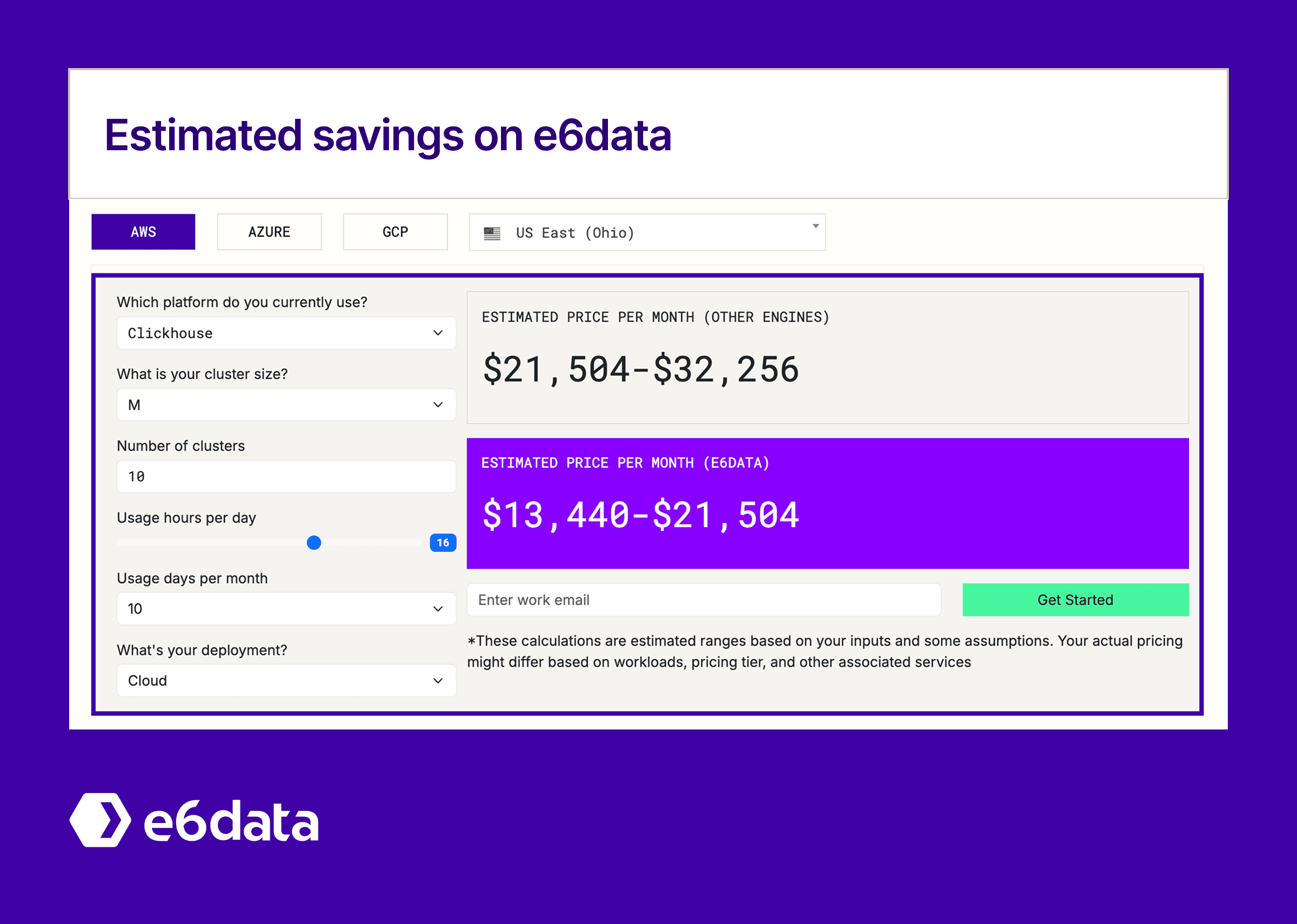
Ready to compare? Run your most resource-intensive ClickHouse queries on a free e6data trial. Most teams see immediate cost improvements on variable analytical workloads while keeping ClickHouse for what it does best.
