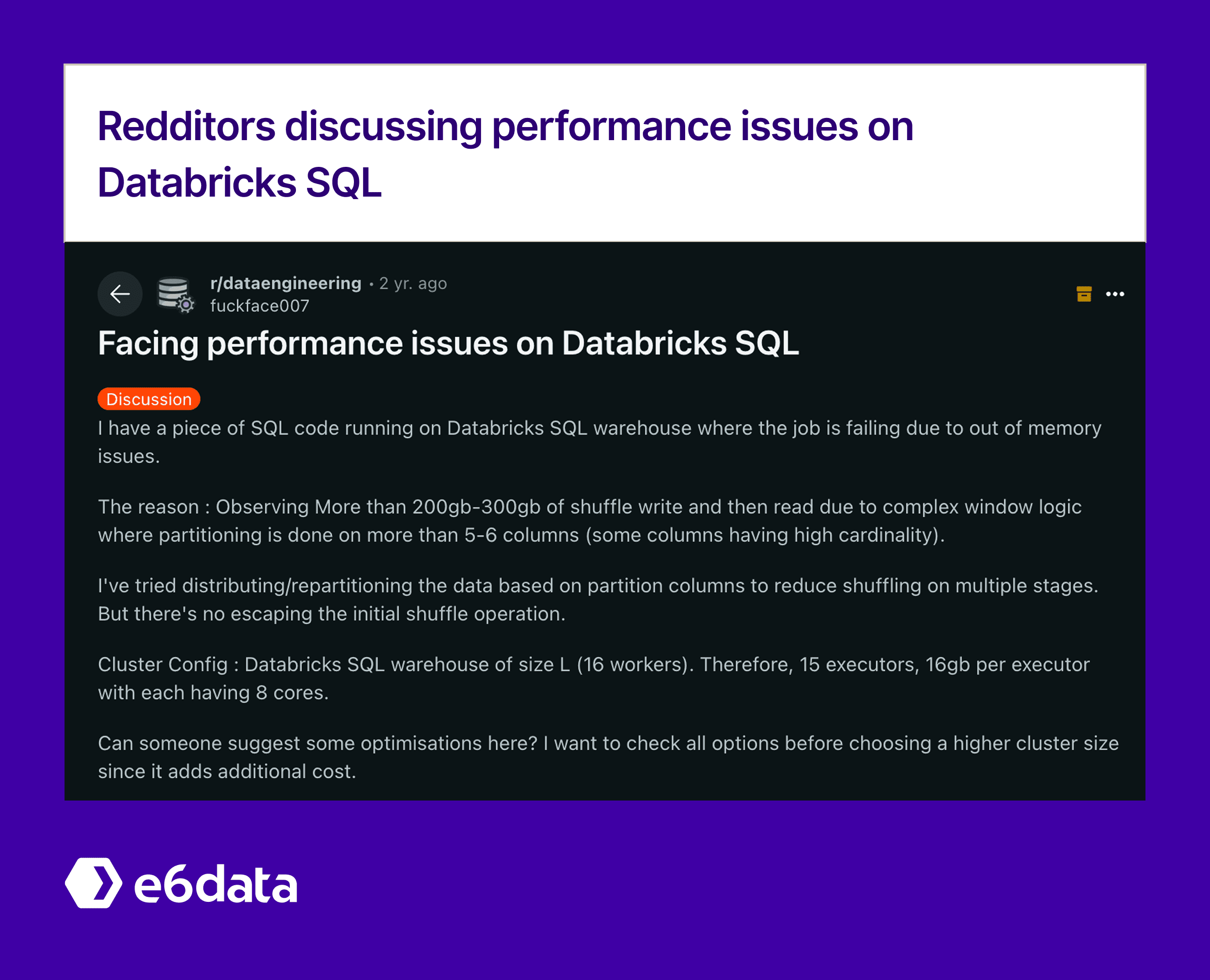
Databricks cost optimization and databricks performance tuning are critical for enterprise data teams managing large-scale analytics workloads. According to Databricks' 2024 State of Data & AI Report, organizations implementing comprehensive databricks performance optimization strategies can achieve significant cost reductions and query performance improvements.
Modern Databricks clusters face performance challenges as data volumes grow exponentially. Enterprise data engineers working with databricks delta lake architectures report that poorly optimized databricks spark queries can consume substantially more DBUs than necessary, directly impacting both operational costs and user experience.
Databricks Performance Optimization Metrics and Thresholds
Based on Databricks Runtime Performance Benchmarks, these databricks cluster performance indicators help identify optimization opportunities across workloads:
Databricks SQL query latency · Optimization Threshold: >30s for BI dashboards · Required Action: Implement databricks liquid clustering and delta lake Z-ordering
Data skipping efficiency · Optimization Threshold: <70% files eliminated · Required Action: Optimize databricks delta tables layout and statistics collection
Delta Cache hit ratio · Optimization Threshold: <60% for repeated queries · Required Action: Configure databricks cluster cache settings and Unity Catalog caching
Cluster CPU utilization · Optimization Threshold: >85% sustained load · Required Action: Scale databricks cluster resources or optimize Spark SQL parallelism
Shuffle operation volume · Optimization Threshold: >1GB per query · Required Action: Review databricks spark join strategies and broadcast hints
Concurrent query queue time · Optimization Threshold: >10s during peak hours · Required Action: Enable databricks sql serverless or implement workload isolation
DBU consumption variance · Optimization Threshold: >150% of cost baseline · Required Action: Audit spark databricks execution plans and implement databricks cost optimization
BI Dashboard Optimization Tactics
1. Implement Z-Ordering for Sub-Second Query Response
When to apply: Deploy Z-ordering when tables exceed 1GB and databricks sql dashboards filter on multiple dimensions like customer_id, date_range, and product_category. According to Databricks Delta Lake Performance Guide, traditional partitioning fails when users query across various column combinations. Z-ordering excels on high-cardinality columns appearing frequently in WHERE clauses, particularly for sql dashboard queries filtering on 2+ columns regularly.
How to implement: Z-ordering co-locates related data using space-filling curves, dramatically improving data skipping efficiency for multi-dimensional queries. Enterprise implementations can achieve significant performance improvements on point lookups and range scans when Z-ordering is implemented correctly.
-- Optimize sales table for common BI query patterns
OPTIMIZE sales_fact
ZORDER BY (customer_id, transaction_date, product_category);

-- Enable auto-optimize for ongoing maintenance
ALTER TABLE sales_fact
SET TBLPROPERTIES (
  'delta.autoOptimize.optimizeWrite' = 'true',
  'delta.autoOptimize.autoCompact' = 'true'
);

-- Example dashboard query that benefits from Z-ordering
SELECT
    product_category,
    COUNT(*) as transaction_count,
    SUM(amount) as total_revenue
FROM sales_fact
WHERE customer_id IN (12345, 67890, 11111)
    AND transaction_date >= '2024-01-01'
    AND product_category = 'Electronics'
GROUP BY product_category;
-- Optimize sales table for common BI query patterns
OPTIMIZE sales_fact
ZORDER BY (customer_id, transaction_date, product_category);
-- Enable auto-optimize for ongoing maintenance
ALTER TABLE sales_fact
SET TBLPROPERTIES (
'delta.autoOptimize.optimizeWrite' = 'true',
'delta.autoOptimize.autoCompact' = 'true'
);
-- Example dashboard query that benefits from Z-ordering
SELECT
product_category,
COUNT(*) as transaction_count,
SUM(amount) as total_revenue
FROM sales_fact
WHERE customer_id IN (12345, 67890, 11111)
AND transaction_date >= '2024-01-01'
AND product_category = 'Electronics'
GROUP BY product_category;-- Optimize sales table for common BI query patterns
OPTIMIZE sales_fact
ZORDER BY (customer_id, transaction_date, product_category);
-- Enable auto-optimize for ongoing maintenance
ALTER TABLE sales_fact
SET TBLPROPERTIES (
'delta.autoOptimize.optimizeWrite' = 'true',
'delta.autoOptimize.autoCompact' = 'true'
);
-- Example dashboard query that benefits from Z-ordering
SELECT
product_category,
COUNT(*) as transaction_count,
SUM(amount) as total_revenue
FROM sales_fact
WHERE customer_id IN (12345, 67890, 11111)
AND transaction_date >= '2024-01-01'
AND product_category = 'Electronics'
GROUP BY product_category;-- Optimize sales table for common BI query patterns
OPTIMIZE sales_fact
ZORDER BY (customer_id, transaction_date, product_category);
-- Enable auto-optimize for ongoing maintenance
ALTER TABLE sales_fact
SET TBLPROPERTIES (
'delta.autoOptimize.optimizeWrite' = 'true',
'delta.autoOptimize.autoCompact' = 'true'
);
-- Example dashboard query that benefits from Z-ordering
SELECT
product_category,
COUNT(*) as transaction_count,
SUM(amount) as total_revenue
FROM sales_fact
WHERE customer_id IN (12345, 67890, 11111)
AND transaction_date >= '2024-01-01'
AND product_category = 'Electronics'
GROUP BY product_category;Alternatives: Delta Lake Bloom filters for high-cardinality string columns (note: effectiveness is limited and feature availability may vary), databricks liquid clustering for evolving access patterns (note: Liquid Clustering replaces Z-Order and requires Unity Catalog managed tables), or migrating performance-critical queries to e6data for guaranteed sub-second latency without maintenance overhead.
2. Implement Delta Cache for Repetitive Dashboard Queries
When to apply: Implement caching for tables <10GB that are accessed >5 times per hour when dashboard users repeatedly access the same data throughout the day, making caching strategies crucial for maintaining sub-second response times.
How to implement: Databricks IO cache (formerly Delta Cache) stores frequently accessed data on local SSD storage, reducing network I/O and significantly improving query performance for repeated access patterns. IO cache works transparently at the file level and automatically manages cache eviction based on access patterns.
-- Enable Databricks IO cache on cluster
-- Cluster configuration: Advanced Options > Spark Config
spark.databricks.io.cache.enabled true
spark.databricks.io.cache.maxDiskUsage 50g

-- Optional: Use Spark in-memory caching for specific tables (separate from IO cache)
-- CACHE TABLE customer_dim;
-- CACHE TABLE product_dim;

-- Dashboard query leveraging cached dimensions
SELECT
    p.product_name,
    c.customer_segment,
    COUNT(*) as order_count,
    SUM(o.order_value) as total_revenue
FROM orders_fact o
JOIN customer_dim c ON o.customer_id = c.customer_id  -- Benefits from IO cache
JOIN product_dim p ON o.product_id = p.product_id    -- Benefits from IO cache
WHERE o.order_date >= CURRENT_DATE - INTERVAL 30 DAYS
GROUP BY p.product_name, c.customer_segment
HAVING COUNT(*) >= 10;
-- Enable Databricks IO cache on cluster
-- Cluster configuration: Advanced Options > Spark Config
spark.databricks.io.cache.enabled true
spark.databricks.io.cache.maxDiskUsage 50g
-- Optional: Use Spark in-memory caching for specific tables (separate from IO cache)
-- CACHE TABLE customer_dim;
-- CACHE TABLE product_dim;
-- Dashboard query leveraging cached dimensions
SELECT
p.product_name,
c.customer_segment,
COUNT(*) as order_count,
SUM(o.order_value) as total_revenue
FROM orders_fact o
JOIN customer_dim c ON o.customer_id = c.customer_id -- Benefits from IO cache
JOIN product_dim p ON o.product_id = p.product_id -- Benefits from IO cache
WHERE o.order_date >= CURRENT_DATE - INTERVAL 30 DAYS
GROUP BY p.product_name, c.customer_segment
HAVING COUNT(*) >= 10;-- Enable Databricks IO cache on cluster
-- Cluster configuration: Advanced Options > Spark Config
spark.databricks.io.cache.enabled true
spark.databricks.io.cache.maxDiskUsage 50g
-- Optional: Use Spark in-memory caching for specific tables (separate from IO cache)
-- CACHE TABLE customer_dim;
-- CACHE TABLE product_dim;
-- Dashboard query leveraging cached dimensions
SELECT
p.product_name,
c.customer_segment,
COUNT(*) as order_count,
SUM(o.order_value) as total_revenue
FROM orders_fact o
JOIN customer_dim c ON o.customer_id = c.customer_id -- Benefits from IO cache
JOIN product_dim p ON o.product_id = p.product_id -- Benefits from IO cache
WHERE o.order_date >= CURRENT_DATE - INTERVAL 30 DAYS
GROUP BY p.product_name, c.customer_segment
HAVING COUNT(*) >= 10;-- Enable Databricks IO cache on cluster
-- Cluster configuration: Advanced Options > Spark Config
spark.databricks.io.cache.enabled true
spark.databricks.io.cache.maxDiskUsage 50g
-- Optional: Use Spark in-memory caching for specific tables (separate from IO cache)
-- CACHE TABLE customer_dim;
-- CACHE TABLE product_dim;
-- Dashboard query leveraging cached dimensions
SELECT
p.product_name,
c.customer_segment,
COUNT(*) as order_count,
SUM(o.order_value) as total_revenue
FROM orders_fact o
JOIN customer_dim c ON o.customer_id = c.customer_id -- Benefits from IO cache
JOIN product_dim p ON o.product_id = p.product_id -- Benefits from IO cache
WHERE o.order_date >= CURRENT_DATE - INTERVAL 30 DAYS
GROUP BY p.product_name, c.customer_segment
HAVING COUNT(*) >= 10;Alternatives: Result caching for identical queries, or adaptive query execution for dynamic optimization.
3. Optimize Partition Pruning with Predicate Pushdown
When to apply: Partition tables >1GB with predictable access patterns where effective partition pruning can dramatically reduce data scanning for time-based BI reports. Target file sizes of 128MB-1GB within partitions, and ensure partition cardinality is balanced (avoid too many small partitions or too few large ones).
How to implement: The key insight here is avoiding the common mistake where users partition by date but then query across customer segments or regions, resulting in full partition scans. Once you've set up partition elimination correctly, query execution times drop dramatically because Spark only reads relevant partitions rather than scanning the entire table.
-- Create properly partitioned table for BI workloads
CREATE TABLE sales_monthly_partitioned (
    transaction_id BIGINT,
    customer_id BIGINT,
    product_id BIGINT,
    sales_amount DECIMAL(10,2),
    region STRING,
    transaction_timestamp TIMESTAMP
) USING DELTA
PARTITIONED BY (
    transaction_month STRING  -- YYYY-MM format for monthly reports
);

-- Insert with proper partition values
INSERT INTO sales_monthly_partitioned
SELECT
    transaction_id,
    customer_id,
    product_id,
    sales_amount,
    region,
    transaction_timestamp,
    DATE_FORMAT(transaction_timestamp, 'yyyy-MM') as transaction_month
FROM raw_sales_data;

-- BI query with effective partition pruning
SELECT
    region,
    COUNT(*) as transaction_count,
    AVG(sales_amount) as avg_sales
FROM sales_monthly_partitioned
WHERE transaction_month = '2024-12'  -- Partition filter eliminates majority of data
    AND region IN ('North', 'South')
GROUP BY region;
-- Create properly partitioned table for BI workloads
CREATE TABLE sales_monthly_partitioned (
transaction_id BIGINT,
customer_id BIGINT,
product_id BIGINT,
sales_amount DECIMAL(10,2),
region STRING,
transaction_timestamp TIMESTAMP
) USING DELTA
PARTITIONED BY (
transaction_month STRING -- YYYY-MM format for monthly reports
);
-- Insert with proper partition values
INSERT INTO sales_monthly_partitioned
SELECT
transaction_id,
customer_id,
product_id,
sales_amount,
region,
transaction_timestamp,
DATE_FORMAT(transaction_timestamp, 'yyyy-MM') as transaction_month
FROM raw_sales_data;
-- BI query with effective partition pruning
SELECT
region,
COUNT(*) as transaction_count,
AVG(sales_amount) as avg_sales
FROM sales_monthly_partitioned
WHERE transaction_month = '2024-12' -- Partition filter eliminates majority of data
AND region IN ('North', 'South')
GROUP BY region;-- Create properly partitioned table for BI workloads
CREATE TABLE sales_monthly_partitioned (
transaction_id BIGINT,
customer_id BIGINT,
product_id BIGINT,
sales_amount DECIMAL(10,2),
region STRING,
transaction_timestamp TIMESTAMP
) USING DELTA
PARTITIONED BY (
transaction_month STRING -- YYYY-MM format for monthly reports
);
-- Insert with proper partition values
INSERT INTO sales_monthly_partitioned
SELECT
transaction_id,
customer_id,
product_id,
sales_amount,
region,
transaction_timestamp,
DATE_FORMAT(transaction_timestamp, 'yyyy-MM') as transaction_month
FROM raw_sales_data;
-- BI query with effective partition pruning
SELECT
region,
COUNT(*) as transaction_count,
AVG(sales_amount) as avg_sales
FROM sales_monthly_partitioned
WHERE transaction_month = '2024-12' -- Partition filter eliminates majority of data
AND region IN ('North', 'South')
GROUP BY region;-- Create properly partitioned table for BI workloads
CREATE TABLE sales_monthly_partitioned (
transaction_id BIGINT,
customer_id BIGINT,
product_id BIGINT,
sales_amount DECIMAL(10,2),
region STRING,
transaction_timestamp TIMESTAMP
) USING DELTA
PARTITIONED BY (
transaction_month STRING -- YYYY-MM format for monthly reports
);
-- Insert with proper partition values
INSERT INTO sales_monthly_partitioned
SELECT
transaction_id,
customer_id,
product_id,
sales_amount,
region,
transaction_timestamp,
DATE_FORMAT(transaction_timestamp, 'yyyy-MM') as transaction_month
FROM raw_sales_data;
-- BI query with effective partition pruning
SELECT
region,
COUNT(*) as transaction_count,
AVG(sales_amount) as avg_sales
FROM sales_monthly_partitioned
WHERE transaction_month = '2024-12' -- Partition filter eliminates majority of data
AND region IN ('North', 'South')
GROUP BY region;Alternatives: Dynamic partition pruning for complex joins, or liquid clustering for evolving patterns.
4. Enable Serverless SQL for Consistent BI Performance
When to apply: Use serverless for BI workloads with unpredictable usage patterns where response time consistency matters more than absolute performance. Serverless scales well beyond 50 concurrent users and particularly shines for user-facing dashboards that need to eliminate the cold start problem.
How to implement: Serverless SQL eliminates the cold start problem that plagues traditional cluster-based BI deployments by providing instant query execution with automatic scaling based on demand instead of waiting several minutes for cluster startup during peak usage. The beauty of this approach is that it removes the operational overhead of cluster sizing and management while providing predictable query latency.
-- Serverless SQL endpoint configuration (via UI or API)
-- No cluster management required - automatic scaling

-- BI dashboard query on serverless endpoint
WITH monthly_metrics AS (
    SELECT
        DATE_TRUNC('month', order_date) as month,
        customer_segment,
        SUM(order_value) as revenue,
        COUNT(DISTINCT customer_id) as active_customers,
        AVG(order_value) as avg_order_size
    FROM orders_fact o
    JOIN customer_dim c ON o.customer_id = c.customer_id
    WHERE order_date >= '2024-01-01'
    GROUP BY DATE_TRUNC('month', order_date), customer_segment
)
SELECT
    month,
    customer_segment,
    revenue,
    active_customers,
    avg_order_size,
    LAG(revenue) OVER (PARTITION BY customer_segment ORDER BY month) as prev_month_revenue,
    (revenue - LAG(revenue) OVER (PARTITION BY customer_segment ORDER BY month)) /
        LAG(revenue) OVER (PARTITION BY customer_segment ORDER BY month) * 100 as growth_rate
FROM monthly_metrics
ORDER BY month DESC, customer_segment;
-- Serverless SQL endpoint configuration (via UI or API)
-- No cluster management required - automatic scaling
-- BI dashboard query on serverless endpoint
WITH monthly_metrics AS (
SELECT
DATE_TRUNC('month', order_date) as month,
customer_segment,
SUM(order_value) as revenue,
COUNT(DISTINCT customer_id) as active_customers,
AVG(order_value) as avg_order_size
FROM orders_fact o
JOIN customer_dim c ON o.customer_id = c.customer_id
WHERE order_date >= '2024-01-01'
GROUP BY DATE_TRUNC('month', order_date), customer_segment
)
SELECT
month,
customer_segment,
revenue,
active_customers,
avg_order_size,
LAG(revenue) OVER (PARTITION BY customer_segment ORDER BY month) as prev_month_revenue,
(revenue - LAG(revenue) OVER (PARTITION BY customer_segment ORDER BY month)) /
LAG(revenue) OVER (PARTITION BY customer_segment ORDER BY month) * 100 as growth_rate
FROM monthly_metrics
ORDER BY month DESC, customer_segment;-- Serverless SQL endpoint configuration (via UI or API)
-- No cluster management required - automatic scaling
-- BI dashboard query on serverless endpoint
WITH monthly_metrics AS (
SELECT
DATE_TRUNC('month', order_date) as month,
customer_segment,
SUM(order_value) as revenue,
COUNT(DISTINCT customer_id) as active_customers,
AVG(order_value) as avg_order_size
FROM orders_fact o
JOIN customer_dim c ON o.customer_id = c.customer_id
WHERE order_date >= '2024-01-01'
GROUP BY DATE_TRUNC('month', order_date), customer_segment
)
SELECT
month,
customer_segment,
revenue,
active_customers,
avg_order_size,
LAG(revenue) OVER (PARTITION BY customer_segment ORDER BY month) as prev_month_revenue,
(revenue - LAG(revenue) OVER (PARTITION BY customer_segment ORDER BY month)) /
LAG(revenue) OVER (PARTITION BY customer_segment ORDER BY month) * 100 as growth_rate
FROM monthly_metrics
ORDER BY month DESC, customer_segment;-- Serverless SQL endpoint configuration (via UI or API)
-- No cluster management required - automatic scaling
-- BI dashboard query on serverless endpoint
WITH monthly_metrics AS (
SELECT
DATE_TRUNC('month', order_date) as month,
customer_segment,
SUM(order_value) as revenue,
COUNT(DISTINCT customer_id) as active_customers,
AVG(order_value) as avg_order_size
FROM orders_fact o
JOIN customer_dim c ON o.customer_id = c.customer_id
WHERE order_date >= '2024-01-01'
GROUP BY DATE_TRUNC('month', order_date), customer_segment
)
SELECT
month,
customer_segment,
revenue,
active_customers,
avg_order_size,
LAG(revenue) OVER (PARTITION BY customer_segment ORDER BY month) as prev_month_revenue,
(revenue - LAG(revenue) OVER (PARTITION BY customer_segment ORDER BY month)) /
LAG(revenue) OVER (PARTITION BY customer_segment ORDER BY month) * 100 as growth_rate
FROM monthly_metrics
ORDER BY month DESC, customer_segment;Alternatives: Right-sized clusters with auto-scaling, Databricks SQL Pro for guaranteed performance, or e6data for sub-second latency with 1000+ concurrent users without migrating from Databricks.
Ad-hoc Analytics Optimization Tactics
1. Implement Broadcast Joins for Dimension Table Performance
When to apply: Use broadcast joins for tables <200MB joining with fact tables >1GB where large fact table joins with smaller dimension tables create massive shuffle operations that can consume significantly more resources than necessary.
How to implement: Broadcast joins copy small tables to all executors, eliminating network shuffle and dramatically reducing query time for typical star schema queries. Spark's adaptive query execution automatically identifies broadcast opportunities, but you can manually control this behavior for predictable performance. What makes this particularly effective is that broadcast joins work exceptionally well with cached dimension tables, creating a powerful combination for analytical workloads.
-- Configure broadcast join thresholds
SET spark.sql.adaptive.enabled = true;
SET spark.sql.autoBroadcastJoinThreshold = 100MB;
-- Manual broadcast hint for guaranteed behavior (hint table aliases individually)
SELECT
c.customer_segment,
p.product_category,
COUNT(*) as order_count,
SUM(o.order_value) as total_revenue,
AVG(o.order_value) as avg_order_value
FROM orders_fact o
JOIN customer_dim c ON o.customer_id = c.customer_id
JOIN product_dim p ON o.product_id = p.product_id
WHERE o.order_date >= '2024-01-01'
GROUP BY c.customer_segment, p.product_category
HAVING SUM(o.order_value) > 100000;-- Configure broadcast join thresholds
SET spark.sql.adaptive.enabled = true;
SET spark.sql.autoBroadcastJoinThreshold = 100MB;
-- Manual broadcast hint for guaranteed behavior (hint table aliases individually)
SELECT
c.customer_segment,
p.product_category,
COUNT(*) as order_count,
SUM(o.order_value) as total_revenue,
AVG(o.order_value) as avg_order_value
FROM orders_fact o
JOIN customer_dim c ON o.customer_id = c.customer_id
JOIN product_dim p ON o.product_id = p.product_id
WHERE o.order_date >= '2024-01-01'
GROUP BY c.customer_segment, p.product_category
HAVING SUM(o.order_value) > 100000;-- Configure broadcast join thresholds
SET spark.sql.adaptive.enabled = true;
SET spark.sql.autoBroadcastJoinThreshold = 100MB;
-- Manual broadcast hint for guaranteed behavior (hint table aliases individually)
SELECT
c.customer_segment,
p.product_category,
COUNT(*) as order_count,
SUM(o.order_value) as total_revenue,
AVG(o.order_value) as avg_order_value
FROM orders_fact o
JOIN customer_dim c ON o.customer_id = c.customer_id
JOIN product_dim p ON o.product_id = p.product_id
WHERE o.order_date >= '2024-01-01'
GROUP BY c.customer_segment, p.product_category
HAVING SUM(o.order_value) > 100000;-- Configure broadcast join thresholds
SET spark.sql.adaptive.enabled = true;
SET spark.sql.autoBroadcastJoinThreshold = 100MB;
-- Manual broadcast hint for guaranteed behavior (hint table aliases individually)
SELECT
c.customer_segment,
p.product_category,
COUNT(*) as order_count,
SUM(o.order_value) as total_revenue,
AVG(o.order_value) as avg_order_value
FROM orders_fact o
JOIN customer_dim c ON o.customer_id = c.customer_id
JOIN product_dim p ON o.product_id = p.product_id
WHERE o.order_date >= '2024-01-01'
GROUP BY c.customer_segment, p.product_category
HAVING SUM(o.order_value) > 100000;Alternatives: Bucketed joins for predictable data distribution, or sort-merge joins for large-to-large table joins
2. Optimize Window Functions with Proper Partitioning
When to apply: Partition window functions when processing >10M rows where window functions in analytical queries trigger expensive global sorts across the entire dataset, creating memory pressure and long execution times.
How to implement: When you implement proper window partitioning strategies, you transform these operations from cluster-wide sorts to manageable partition-level operations. Partitioning window functions by logical business dimensions like customer_id or region substantially reduces memory usage while maintaining result accuracy. Here's where it gets interesting: combining window partitioning with Z-ordering creates significant performance synergies for ranking and aggregation operations.
-- Inefficient: Global sorting across entire dataset
SELECT
    customer_id,
    order_date,
    order_value,
    ROW_NUMBER() OVER (ORDER BY order_value DESC) as global_rank  -- Expensive!
FROM orders_fact;

-- Optimized: Partition-aware window functions
SELECT
    customer_id,
    order_date,
    order_value,
    SUM(order_value) OVER (
        PARTITION BY customer_id
        ORDER BY order_date
        ROWS BETWEEN 6 PRECEDING AND CURRENT ROW
    ) as rolling_7day_total,
    ROW_NUMBER() OVER (
        PARTITION BY customer_id
        ORDER BY order_value DESC
    ) as customer_order_rank,
    DENSE_RANK() OVER (
        PARTITION BY DATE_TRUNC('month', order_date)
        ORDER BY order_value DESC
    ) as monthly_rank
FROM orders_fact
WHERE order_date >= '2024-01-01';

-- Advanced: Optimize table layout for window operations
OPTIMIZE orders_fact
ZORDER BY (customer_id, order_date);
-- Inefficient: Global sorting across entire dataset
SELECT
customer_id,
order_date,
order_value,
ROW_NUMBER() OVER (ORDER BY order_value DESC) as global_rank -- Expensive!
FROM orders_fact;
-- Optimized: Partition-aware window functions
SELECT
customer_id,
order_date,
order_value,
SUM(order_value) OVER (
PARTITION BY customer_id
ORDER BY order_date
ROWS BETWEEN 6 PRECEDING AND CURRENT ROW
) as rolling_7day_total,
ROW_NUMBER() OVER (
PARTITION BY customer_id
ORDER BY order_value DESC
) as customer_order_rank,
DENSE_RANK() OVER (
PARTITION BY DATE_TRUNC('month', order_date)
ORDER BY order_value DESC
) as monthly_rank
FROM orders_fact
WHERE order_date >= '2024-01-01';
-- Advanced: Optimize table layout for window operations
OPTIMIZE orders_fact
ZORDER BY (customer_id, order_date);-- Inefficient: Global sorting across entire dataset
SELECT
customer_id,
order_date,
order_value,
ROW_NUMBER() OVER (ORDER BY order_value DESC) as global_rank -- Expensive!
FROM orders_fact;
-- Optimized: Partition-aware window functions
SELECT
customer_id,
order_date,
order_value,
SUM(order_value) OVER (
PARTITION BY customer_id
ORDER BY order_date
ROWS BETWEEN 6 PRECEDING AND CURRENT ROW
) as rolling_7day_total,
ROW_NUMBER() OVER (
PARTITION BY customer_id
ORDER BY order_value DESC
) as customer_order_rank,
DENSE_RANK() OVER (
PARTITION BY DATE_TRUNC('month', order_date)
ORDER BY order_value DESC
) as monthly_rank
FROM orders_fact
WHERE order_date >= '2024-01-01';
-- Advanced: Optimize table layout for window operations
OPTIMIZE orders_fact
ZORDER BY (customer_id, order_date);-- Inefficient: Global sorting across entire dataset
SELECT
customer_id,
order_date,
order_value,
ROW_NUMBER() OVER (ORDER BY order_value DESC) as global_rank -- Expensive!
FROM orders_fact;
-- Optimized: Partition-aware window functions
SELECT
customer_id,
order_date,
order_value,
SUM(order_value) OVER (
PARTITION BY customer_id
ORDER BY order_date
ROWS BETWEEN 6 PRECEDING AND CURRENT ROW
) as rolling_7day_total,
ROW_NUMBER() OVER (
PARTITION BY customer_id
ORDER BY order_value DESC
) as customer_order_rank,
DENSE_RANK() OVER (
PARTITION BY DATE_TRUNC('month', order_date)
ORDER BY order_value DESC
) as monthly_rank
FROM orders_fact
WHERE order_date >= '2024-01-01';
-- Advanced: Optimize table layout for window operations
OPTIMIZE orders_fact
ZORDER BY (customer_id, order_date);Alternatives: Pre-aggregated materialized views or repeated calculations, approximate functions like percentile_approx.
3. Leverage Adaptive Query Execution for Dynamic Optimization
When to apply: Enable AQE for all analytical workloads where complex analytical queries with multiple joins and aggregations need automatic optimization without manual intervention.
How to implement: Adaptive Query Execution (AQE) accelerates analytical query performance by making runtime decisions based on actual data statistics rather than pre-execution estimates. What makes this particularly effective is that AQE automatically handles skewed joins, optimizes shuffle partitions, and converts sort-merge joins to broadcast joins when beneficial.
-- Enable comprehensive AQE features
SET spark.sql.adaptive.enabled = true;
SET spark.sql.adaptive.coalescePartitions.enabled = true;
SET spark.sql.adaptive.skewJoin.enabled = true;
SET spark.sql.adaptive.localShuffleReader.enabled = true;

-- Complex analytical query that benefits from AQE
WITH customer_metrics AS (
    SELECT
        c.customer_id,
        c.customer_segment,
        COUNT(*) as order_count,
        SUM(o.order_value) as total_spent,
        MAX(o.order_date) as last_order_date
    FROM customers c
    LEFT JOIN orders o ON c.customer_id = o.customer_id
    WHERE c.registration_date >= '2023-01-01'
    GROUP BY c.customer_id, c.customer_segment
),
segment_analysis AS (
    SELECT
        customer_segment,
        AVG(total_spent) as avg_spent,
        PERCENTILE_CONT(0.9) WITHIN GROUP (ORDER BY total_spent) as p90_spent,
        COUNT(*) as segment_size
    FROM customer_metrics
    GROUP BY customer_segment
)
SELECT
    cm.customer_segment,
    COUNT(*) as high_value_customers,
    AVG(cm.total_spent) as avg_high_value_spent,
    sa.avg_spent as segment_avg
FROM customer_metrics cm
JOIN segment_analysis sa ON cm.customer_segment = sa.customer_segment
WHERE cm.total_spent > sa.p90_spent
GROUP BY cm.customer_segment, sa.avg_spent
ORDER BY high_value_customers DESC;
-- Enable comprehensive AQE features
SET spark.sql.adaptive.enabled = true;
SET spark.sql.adaptive.coalescePartitions.enabled = true;
SET spark.sql.adaptive.skewJoin.enabled = true;
SET spark.sql.adaptive.localShuffleReader.enabled = true;
-- Complex analytical query that benefits from AQE
WITH customer_metrics AS (
SELECT
c.customer_id,
c.customer_segment,
COUNT(*) as order_count,
SUM(o.order_value) as total_spent,
MAX(o.order_date) as last_order_date
FROM customers c
LEFT JOIN orders o ON c.customer_id = o.customer_id
WHERE c.registration_date >= '2023-01-01'
GROUP BY c.customer_id, c.customer_segment
),
segment_analysis AS (
SELECT
customer_segment,
AVG(total_spent) as avg_spent,
PERCENTILE_CONT(0.9) WITHIN GROUP (ORDER BY total_spent) as p90_spent,
COUNT(*) as segment_size
FROM customer_metrics
GROUP BY customer_segment
)
SELECT
cm.customer_segment,
COUNT(*) as high_value_customers,
AVG(cm.total_spent) as avg_high_value_spent,
sa.avg_spent as segment_avg
FROM customer_metrics cm
JOIN segment_analysis sa ON cm.customer_segment = sa.customer_segment
WHERE cm.total_spent > sa.p90_spent
GROUP BY cm.customer_segment, sa.avg_spent
ORDER BY high_value_customers DESC;-- Enable comprehensive AQE features
SET spark.sql.adaptive.enabled = true;
SET spark.sql.adaptive.coalescePartitions.enabled = true;
SET spark.sql.adaptive.skewJoin.enabled = true;
SET spark.sql.adaptive.localShuffleReader.enabled = true;
-- Complex analytical query that benefits from AQE
WITH customer_metrics AS (
SELECT
c.customer_id,
c.customer_segment,
COUNT(*) as order_count,
SUM(o.order_value) as total_spent,
MAX(o.order_date) as last_order_date
FROM customers c
LEFT JOIN orders o ON c.customer_id = o.customer_id
WHERE c.registration_date >= '2023-01-01'
GROUP BY c.customer_id, c.customer_segment
),
segment_analysis AS (
SELECT
customer_segment,
AVG(total_spent) as avg_spent,
PERCENTILE_CONT(0.9) WITHIN GROUP (ORDER BY total_spent) as p90_spent,
COUNT(*) as segment_size
FROM customer_metrics
GROUP BY customer_segment
)
SELECT
cm.customer_segment,
COUNT(*) as high_value_customers,
AVG(cm.total_spent) as avg_high_value_spent,
sa.avg_spent as segment_avg
FROM customer_metrics cm
JOIN segment_analysis sa ON cm.customer_segment = sa.customer_segment
WHERE cm.total_spent > sa.p90_spent
GROUP BY cm.customer_segment, sa.avg_spent
ORDER BY high_value_customers DESC;-- Enable comprehensive AQE features
SET spark.sql.adaptive.enabled = true;
SET spark.sql.adaptive.coalescePartitions.enabled = true;
SET spark.sql.adaptive.skewJoin.enabled = true;
SET spark.sql.adaptive.localShuffleReader.enabled = true;
-- Complex analytical query that benefits from AQE
WITH customer_metrics AS (
SELECT
c.customer_id,
c.customer_segment,
COUNT(*) as order_count,
SUM(o.order_value) as total_spent,
MAX(o.order_date) as last_order_date
FROM customers c
LEFT JOIN orders o ON c.customer_id = o.customer_id
WHERE c.registration_date >= '2023-01-01'
GROUP BY c.customer_id, c.customer_segment
),
segment_analysis AS (
SELECT
customer_segment,
AVG(total_spent) as avg_spent,
PERCENTILE_CONT(0.9) WITHIN GROUP (ORDER BY total_spent) as p90_spent,
COUNT(*) as segment_size
FROM customer_metrics
GROUP BY customer_segment
)
SELECT
cm.customer_segment,
COUNT(*) as high_value_customers,
AVG(cm.total_spent) as avg_high_value_spent,
sa.avg_spent as segment_avg
FROM customer_metrics cm
JOIN segment_analysis sa ON cm.customer_segment = sa.customer_segment
WHERE cm.total_spent > sa.p90_spent
GROUP BY cm.customer_segment, sa.avg_spent
ORDER BY high_value_customers DESC;Alternatives: Manual join hints and partition tuning, cost-based optimizer statistics collection, or e6data's lakehouse query engine's query optimization that eliminates manual tuning entirely.
4. Implement Columnar Statistics for Intelligent Data Skipping
When to apply: Collect statistics for tables >1GB with selective filter patterns where Delta Lake's column-level statistics can enable sophisticated data skipping that goes beyond basic partition pruning.
How to implement: When you collect statistics on frequently filtered columns, the query optimizer can skip entire files without reading them, substantially reducing I/O for selective analytical queries. Here's what happens next: the Delta Log maintains min/max statistics for each data file, allowing the query engine to eliminate files that don't contain relevant data before any actual data reading occurs. What makes this particularly effective is combining statistics with Z-ordering for maximum data skipping efficiency.
-- Delta Lake maintains file-level min/max statistics automatically
-- Focus on collecting table-level statistics for cost-based optimization

-- Analyze table to compute statistics
ANALYZE TABLE sales_fact COMPUTE STATISTICS FOR ALL COLUMNS;

-- Query that benefits from data skipping
SELECT
    customer_segment,
    product_category,
    SUM(sales_amount) as total_sales,
    COUNT(DISTINCT customer_id) as unique_customers
FROM sales_fact s
JOIN customer_dim c ON s.customer_id = c.customer_id
WHERE s.sales_amount > 1000  -- Statistics enable file skipping
    AND s.transaction_date BETWEEN '2024-11-01' AND '2024-11-30'
    AND c.customer_segment = 'Enterprise'
GROUP BY customer_segment, product_category;
-- Delta Lake maintains file-level min/max statistics automatically
-- Focus on collecting table-level statistics for cost-based optimization
-- Analyze table to compute statistics
ANALYZE TABLE sales_fact COMPUTE STATISTICS FOR ALL COLUMNS;
-- Query that benefits from data skipping
SELECT
customer_segment,
product_category,
SUM(sales_amount) as total_sales,
COUNT(DISTINCT customer_id) as unique_customers
FROM sales_fact s
JOIN customer_dim c ON s.customer_id = c.customer_id
WHERE s.sales_amount > 1000 -- Statistics enable file skipping
AND s.transaction_date BETWEEN '2024-11-01' AND '2024-11-30'
AND c.customer_segment = 'Enterprise'
GROUP BY customer_segment, product_category;-- Delta Lake maintains file-level min/max statistics automatically
-- Focus on collecting table-level statistics for cost-based optimization
-- Analyze table to compute statistics
ANALYZE TABLE sales_fact COMPUTE STATISTICS FOR ALL COLUMNS;
-- Query that benefits from data skipping
SELECT
customer_segment,
product_category,
SUM(sales_amount) as total_sales,
COUNT(DISTINCT customer_id) as unique_customers
FROM sales_fact s
JOIN customer_dim c ON s.customer_id = c.customer_id
WHERE s.sales_amount > 1000 -- Statistics enable file skipping
AND s.transaction_date BETWEEN '2024-11-01' AND '2024-11-30'
AND c.customer_segment = 'Enterprise'
GROUP BY customer_segment, product_category;-- Delta Lake maintains file-level min/max statistics automatically
-- Focus on collecting table-level statistics for cost-based optimization
-- Analyze table to compute statistics
ANALYZE TABLE sales_fact COMPUTE STATISTICS FOR ALL COLUMNS;
-- Query that benefits from data skipping
SELECT
customer_segment,
product_category,
SUM(sales_amount) as total_sales,
COUNT(DISTINCT customer_id) as unique_customers
FROM sales_fact s
JOIN customer_dim c ON s.customer_id = c.customer_id
WHERE s.sales_amount > 1000 -- Statistics enable file skipping
AND s.transaction_date BETWEEN '2024-11-01' AND '2024-11-30'
AND c.customer_segment = 'Enterprise'
GROUP BY customer_segment, product_category;Alternatives: Bloom filters for high-cardinality columns, manual file organization strategies, or e6data's query engine's automatic data skipping optimization.
5. Deploy Predictive I/O for Large Scan Operations
When to apply: Enable predictive I/O for sequential scan patterns >10GB where many analytical queries follow predictable access patterns, allowing the storage layer to anticipate data needs and reduce wait times.
How to implement: Predictive I/O pre-fetches data that's likely to be accessed based on query patterns, reducing latency for large analytical scans. You'll find that predictive I/O works exceptionally well with time-series analysis and sequential data processing where queries typically access adjacent data ranges. Once you've enabled predictive optimization, scan-heavy analytical queries see meaningful latency reduction due to reduced I/O wait times.
-- Enable IO cache for improved scan performance
SET spark.databricks.io.cache.enabled = true;
-- Note: Read-ahead and prefetch optimizations are handled automatically

-- Time-series analysis that benefits from predictive I/O
WITH daily_metrics AS (
    SELECT
        transaction_date,
        COUNT(*) as transaction_count,
        SUM(amount) as daily_revenue,
        AVG(amount) as avg_transaction_size,
        COUNT(DISTINCT customer_id) as active_customers
    FROM transactions
    WHERE transaction_date >= '2024-01-01'
    GROUP BY transaction_date
),
moving_averages AS (
    SELECT
        transaction_date,
        daily_revenue,
        AVG(daily_revenue) OVER (
            ORDER BY transaction_date
            ROWS BETWEEN 6 PRECEDING AND CURRENT ROW
        ) as ma_7day,
        AVG(daily_revenue) OVER (
            ORDER BY transaction_date
            ROWS BETWEEN 29 PRECEDING AND CURRENT ROW
        ) as ma_30day
    FROM daily_metrics
)
SELECT
    transaction_date,
    daily_revenue,
    ma_7day,
    ma_30day,
    (daily_revenue - ma_7day) / ma_7day * 100 as deviation_from_7day,
    CASE
        WHEN daily_revenue > ma_30day * 1.2 THEN 'High Performance'
        WHEN daily_revenue < ma_30day * 0.8 THEN 'Low Performance'
        ELSE 'Normal'
    END as performance_category
FROM moving_averages
ORDER BY transaction_date DESC;
-- Enable IO cache for improved scan performance
SET spark.databricks.io.cache.enabled = true;
-- Note: Read-ahead and prefetch optimizations are handled automatically
-- Time-series analysis that benefits from predictive I/O
WITH daily_metrics AS (
SELECT
transaction_date,
COUNT(*) as transaction_count,
SUM(amount) as daily_revenue,
AVG(amount) as avg_transaction_size,
COUNT(DISTINCT customer_id) as active_customers
FROM transactions
WHERE transaction_date >= '2024-01-01'
GROUP BY transaction_date
),
moving_averages AS (
SELECT
transaction_date,
daily_revenue,
AVG(daily_revenue) OVER (
ORDER BY transaction_date
ROWS BETWEEN 6 PRECEDING AND CURRENT ROW
) as ma_7day,
AVG(daily_revenue) OVER (
ORDER BY transaction_date
ROWS BETWEEN 29 PRECEDING AND CURRENT ROW
) as ma_30day
FROM daily_metrics
)
SELECT
transaction_date,
daily_revenue,
ma_7day,
ma_30day,
(daily_revenue - ma_7day) / ma_7day * 100 as deviation_from_7day,
CASE
WHEN daily_revenue > ma_30day * 1.2 THEN 'High Performance'
WHEN daily_revenue < ma_30day * 0.8 THEN 'Low Performance'
ELSE 'Normal'
END as performance_category
FROM moving_averages
ORDER BY transaction_date DESC;-- Enable IO cache for improved scan performance
SET spark.databricks.io.cache.enabled = true;
-- Note: Read-ahead and prefetch optimizations are handled automatically
-- Time-series analysis that benefits from predictive I/O
WITH daily_metrics AS (
SELECT
transaction_date,
COUNT(*) as transaction_count,
SUM(amount) as daily_revenue,
AVG(amount) as avg_transaction_size,
COUNT(DISTINCT customer_id) as active_customers
FROM transactions
WHERE transaction_date >= '2024-01-01'
GROUP BY transaction_date
),
moving_averages AS (
SELECT
transaction_date,
daily_revenue,
AVG(daily_revenue) OVER (
ORDER BY transaction_date
ROWS BETWEEN 6 PRECEDING AND CURRENT ROW
) as ma_7day,
AVG(daily_revenue) OVER (
ORDER BY transaction_date
ROWS BETWEEN 29 PRECEDING AND CURRENT ROW
) as ma_30day
FROM daily_metrics
)
SELECT
transaction_date,
daily_revenue,
ma_7day,
ma_30day,
(daily_revenue - ma_7day) / ma_7day * 100 as deviation_from_7day,
CASE
WHEN daily_revenue > ma_30day * 1.2 THEN 'High Performance'
WHEN daily_revenue < ma_30day * 0.8 THEN 'Low Performance'
ELSE 'Normal'
END as performance_category
FROM moving_averages
ORDER BY transaction_date DESC;-- Enable IO cache for improved scan performance
SET spark.databricks.io.cache.enabled = true;
-- Note: Read-ahead and prefetch optimizations are handled automatically
-- Time-series analysis that benefits from predictive I/O
WITH daily_metrics AS (
SELECT
transaction_date,
COUNT(*) as transaction_count,
SUM(amount) as daily_revenue,
AVG(amount) as avg_transaction_size,
COUNT(DISTINCT customer_id) as active_customers
FROM transactions
WHERE transaction_date >= '2024-01-01'
GROUP BY transaction_date
),
moving_averages AS (
SELECT
transaction_date,
daily_revenue,
AVG(daily_revenue) OVER (
ORDER BY transaction_date
ROWS BETWEEN 6 PRECEDING AND CURRENT ROW
) as ma_7day,
AVG(daily_revenue) OVER (
ORDER BY transaction_date
ROWS BETWEEN 29 PRECEDING AND CURRENT ROW
) as ma_30day
FROM daily_metrics
)
SELECT
transaction_date,
daily_revenue,
ma_7day,
ma_30day,
(daily_revenue - ma_7day) / ma_7day * 100 as deviation_from_7day,
CASE
WHEN daily_revenue > ma_30day * 1.2 THEN 'High Performance'
WHEN daily_revenue < ma_30day * 0.8 THEN 'Low Performance'
ELSE 'Normal'
END as performance_category
FROM moving_averages
ORDER BY transaction_date DESC;Alternatives: Manual data pre-loading strategies, or result caching for repeated queries.
ETL/Streaming Optimization Tactics
1. Optimize Auto Loader for High-Throughput Ingestion
When to apply: Optimize Auto Loader for ingestion rates >1GB/hour where default configurations often underperform for high-volume ETL workloads and you need efficient incremental data ingestion.
How to implement: When you optimize Auto Loader settings for your specific data patterns, you can achieve significant throughput improvements while maintaining exactly-once processing semantics. The key insight here is that Auto Loader performance depends heavily on file size, arrival patterns, and parallelism configuration. What makes this particularly effective is combining Auto Loader with Delta Lake's merge operations for upsert-heavy scenarios common in enterprise ETL pipelines.
-- Optimized Auto Loader configuration for high-throughput ingestion
CREATE OR REFRESH STREAMING LIVE TABLE raw_events_optimized
AS SELECT *
FROM cloud_files(
  "s3://your-bucket/events/",
  "json",
  map(
    "cloudFiles.format", "json",
    "cloudFiles.schemaLocation", "s3://your-bucket/schemas/events",
    "cloudFiles.inferColumnTypes", "true",
    "cloudFiles.schemaEvolutionMode", "addNewColumns",
    "cloudFiles.maxFilesPerTrigger", "1000",        -- Optimize for throughput
    "cloudFiles.maxBytesPerTrigger", "1GB",         -- Control batch size
    "cloudFiles.useNotifications", "true",          -- Enable event notifications
    "cloudFiles.validateOptions", "false"           -- Skip validation for speed
  )
);

-- DLT CDC pattern for upsert operations
APPLY CHANGES INTO LIVE.events_processed
FROM STREAM(LIVE.raw_events_optimized)
KEYS (event_id)
SEQUENCE BY event_timestamp
COLUMNS * EXCEPT (event_timestamp)
STORED AS SCD TYPE 1;
-- Optimized Auto Loader configuration for high-throughput ingestion
CREATE OR REFRESH STREAMING LIVE TABLE raw_events_optimized
AS SELECT *
FROM cloud_files(
"s3://your-bucket/events/",
"json",
map(
"cloudFiles.format", "json",
"cloudFiles.schemaLocation", "s3://your-bucket/schemas/events",
"cloudFiles.inferColumnTypes", "true",
"cloudFiles.schemaEvolutionMode", "addNewColumns",
"cloudFiles.maxFilesPerTrigger", "1000", -- Optimize for throughput
"cloudFiles.maxBytesPerTrigger", "1GB", -- Control batch size
"cloudFiles.useNotifications", "true", -- Enable event notifications
"cloudFiles.validateOptions", "false" -- Skip validation for speed
)
);
-- DLT CDC pattern for upsert operations
APPLY CHANGES INTO LIVE.events_processed
FROM STREAM(LIVE.raw_events_optimized)
KEYS (event_id)
SEQUENCE BY event_timestamp
COLUMNS * EXCEPT (event_timestamp)
STORED AS SCD TYPE 1;-- Optimized Auto Loader configuration for high-throughput ingestion
CREATE OR REFRESH STREAMING LIVE TABLE raw_events_optimized
AS SELECT *
FROM cloud_files(
"s3://your-bucket/events/",
"json",
map(
"cloudFiles.format", "json",
"cloudFiles.schemaLocation", "s3://your-bucket/schemas/events",
"cloudFiles.inferColumnTypes", "true",
"cloudFiles.schemaEvolutionMode", "addNewColumns",
"cloudFiles.maxFilesPerTrigger", "1000", -- Optimize for throughput
"cloudFiles.maxBytesPerTrigger", "1GB", -- Control batch size
"cloudFiles.useNotifications", "true", -- Enable event notifications
"cloudFiles.validateOptions", "false" -- Skip validation for speed
)
);
-- DLT CDC pattern for upsert operations
APPLY CHANGES INTO LIVE.events_processed
FROM STREAM(LIVE.raw_events_optimized)
KEYS (event_id)
SEQUENCE BY event_timestamp
COLUMNS * EXCEPT (event_timestamp)
STORED AS SCD TYPE 1;-- Optimized Auto Loader configuration for high-throughput ingestion
CREATE OR REFRESH STREAMING LIVE TABLE raw_events_optimized
AS SELECT *
FROM cloud_files(
"s3://your-bucket/events/",
"json",
map(
"cloudFiles.format", "json",
"cloudFiles.schemaLocation", "s3://your-bucket/schemas/events",
"cloudFiles.inferColumnTypes", "true",
"cloudFiles.schemaEvolutionMode", "addNewColumns",
"cloudFiles.maxFilesPerTrigger", "1000", -- Optimize for throughput
"cloudFiles.maxBytesPerTrigger", "1GB", -- Control batch size
"cloudFiles.useNotifications", "true", -- Enable event notifications
"cloudFiles.validateOptions", "false" -- Skip validation for speed
)
);
-- DLT CDC pattern for upsert operations
APPLY CHANGES INTO LIVE.events_processed
FROM STREAM(LIVE.raw_events_optimized)
KEYS (event_id)
SEQUENCE BY event_timestamp
COLUMNS * EXCEPT (event_timestamp)
STORED AS SCD TYPE 1;Alternatives: Delta Live Tables for complex pipelines, Kafka integration for real-time streams, or e6data's real-time streaming ingest with guaranteed throughput SLAs.
2. Implement Z-Ordering for ETL Output Tables
When to apply: Apply Z-ordering to ETL output tables >1GB accessed by multiple downstream consumers where ETL processes create tables with multiple access patterns, making traditional partitioning insufficient for downstream analytical queries.
How to implement: Z-ordering optimizes data layout for multiple columns simultaneously, improving query performance for various analytical access patterns without sacrificing ETL throughput. You'll find that implementing Z-ordering during ETL write operations eliminates the need for separate optimization jobs while ensuring optimal performance for downstream consumers. Here's where it gets interesting: combining Z-ordering with Delta Lake's write optimization features creates a powerful foundation for both ETL efficiency and query performance.
-- ETL process with integrated Z-ordering
CREATE OR REPLACE TABLE customer_transactions_optimized
USING DELTA
LOCATION 's3://your-bucket/optimized/customer_transactions'
TBLPROPERTIES (
    'delta.autoOptimize.optimizeWrite' = 'true',
    'delta.autoOptimize.autoCompact' = 'true'
);

-- ETL transformation with Z-ordering
INSERT INTO customer_transactions_optimized
SELECT
    t.transaction_id,
    t.customer_id,
    c.customer_segment,
    t.transaction_date,
    t.amount,
    t.product_category,
    CURRENT_TIMESTAMP() as etl_processed_time
FROM raw_transactions t
JOIN customer_master c ON t.customer_id = c.customer_id
WHERE t.transaction_date >= '2024-12-01';

-- Apply Z-ordering after ETL batch completion
-- Note: OPTIMIZE consumes DBUs and should be scheduled, not run on streaming tables
-- Important: Z-Order and Liquid Clustering cannot be used together
OPTIMIZE customer_transactions_optimized
ZORDER BY (customer_id, transaction_date, product_category);

-- Vacuum old files to reclaim storage
-- Warning: Setting retention < 7 days requires disabling retention check and has data loss risk
VACUUM customer_transactions_optimized RETAIN 168 HOURS;
-- ETL process with integrated Z-ordering
CREATE OR REPLACE TABLE customer_transactions_optimized
USING DELTA
LOCATION 's3://your-bucket/optimized/customer_transactions'
TBLPROPERTIES (
'delta.autoOptimize.optimizeWrite' = 'true',
'delta.autoOptimize.autoCompact' = 'true'
);
-- ETL transformation with Z-ordering
INSERT INTO customer_transactions_optimized
SELECT
t.transaction_id,
t.customer_id,
c.customer_segment,
t.transaction_date,
t.amount,
t.product_category,
CURRENT_TIMESTAMP() as etl_processed_time
FROM raw_transactions t
JOIN customer_master c ON t.customer_id = c.customer_id
WHERE t.transaction_date >= '2024-12-01';
-- Apply Z-ordering after ETL batch completion
-- Note: OPTIMIZE consumes DBUs and should be scheduled, not run on streaming tables
-- Important: Z-Order and Liquid Clustering cannot be used together
OPTIMIZE customer_transactions_optimized
ZORDER BY (customer_id, transaction_date, product_category);
-- Vacuum old files to reclaim storage
-- Warning: Setting retention < 7 days requires disabling retention check and has data loss risk
VACUUM customer_transactions_optimized RETAIN 168 HOURS;-- ETL process with integrated Z-ordering
CREATE OR REPLACE TABLE customer_transactions_optimized
USING DELTA
LOCATION 's3://your-bucket/optimized/customer_transactions'
TBLPROPERTIES (
'delta.autoOptimize.optimizeWrite' = 'true',
'delta.autoOptimize.autoCompact' = 'true'
);
-- ETL transformation with Z-ordering
INSERT INTO customer_transactions_optimized
SELECT
t.transaction_id,
t.customer_id,
c.customer_segment,
t.transaction_date,
t.amount,
t.product_category,
CURRENT_TIMESTAMP() as etl_processed_time
FROM raw_transactions t
JOIN customer_master c ON t.customer_id = c.customer_id
WHERE t.transaction_date >= '2024-12-01';
-- Apply Z-ordering after ETL batch completion
-- Note: OPTIMIZE consumes DBUs and should be scheduled, not run on streaming tables
-- Important: Z-Order and Liquid Clustering cannot be used together
OPTIMIZE customer_transactions_optimized
ZORDER BY (customer_id, transaction_date, product_category);
-- Vacuum old files to reclaim storage
-- Warning: Setting retention < 7 days requires disabling retention check and has data loss risk
VACUUM customer_transactions_optimized RETAIN 168 HOURS;-- ETL process with integrated Z-ordering
CREATE OR REPLACE TABLE customer_transactions_optimized
USING DELTA
LOCATION 's3://your-bucket/optimized/customer_transactions'
TBLPROPERTIES (
'delta.autoOptimize.optimizeWrite' = 'true',
'delta.autoOptimize.autoCompact' = 'true'
);
-- ETL transformation with Z-ordering
INSERT INTO customer_transactions_optimized
SELECT
t.transaction_id,
t.customer_id,
c.customer_segment,
t.transaction_date,
t.amount,
t.product_category,
CURRENT_TIMESTAMP() as etl_processed_time
FROM raw_transactions t
JOIN customer_master c ON t.customer_id = c.customer_id
WHERE t.transaction_date >= '2024-12-01';
-- Apply Z-ordering after ETL batch completion
-- Note: OPTIMIZE consumes DBUs and should be scheduled, not run on streaming tables
-- Important: Z-Order and Liquid Clustering cannot be used together
OPTIMIZE customer_transactions_optimized
ZORDER BY (customer_id, transaction_date, product_category);
-- Vacuum old files to reclaim storage
-- Warning: Setting retention < 7 days requires disabling retention check and has data loss risk
VACUUM customer_transactions_optimized RETAIN 168 HOURS;Alternatives: Liquid clustering for evolving access patterns, or partition-based organization.
3. Leverage Delta Lake Change Data Feed for Incremental Processing
When to apply: Implement CDF for tables with <50% daily change rates and downstream dependency chains where efficient incremental ETL is needed by tracking only changed records rather than reprocessing entire datasets.
How to implement: Change Data Feed (CDF) enables you to dramatically reduce ETL runtime while maintaining data consistency across downstream systems. The beauty of this approach is that CDF automatically captures insert, update, and delete operations with versioning information, allowing downstream processes to apply changes incrementally. What makes this particularly effective is combining CDF with streaming processing for near real-time data pipeline updates.
-- Enable Change Data Feed on source table
ALTER TABLE customer_master
SET TBLPROPERTIES (delta.enableChangeDataFeed = true);

-- For streaming CDF consumption, use DataFrame API with readChangeData
-- Note: table_changes() is for batch processing only
-- Example in Python/PySpark:
-- df = spark.readStream.format("delta") \
--   .option("readChangeData", "true") \
--   .table("customer_master") \
--   .where("_change_type in ('insert','update_postimage')")

-- Alternative: Use DLT APPLY CHANGES for CDC patterns
APPLY CHANGES INTO LIVE.customer_analytics_summary
FROM STREAM(LIVE.customer_master)
KEYS (customer_id)
SEQUENCE BY _commit_timestamp
COLUMNS * EXCEPT (_change_type, _commit_version, _commit_timestamp)
STORED AS SCD TYPE 1;

-- Apply incremental changes to downstream analytics table
MERGE INTO customer_analytics_summary t
USING customer_changes_stream s
ON t.customer_id = s.customer_id
WHEN MATCHED AND s._change_type = 'update_postimage' THEN
    UPDATE SET
        t.customer_segment = s.customer_segment,
        t.last_transaction_date = s.last_transaction_date,
        t.lifetime_value = s.lifetime_value,
        t.updated_timestamp = CURRENT_TIMESTAMP()
WHEN NOT MATCHED AND s._change_type = 'insert' THEN
    INSERT (customer_id, customer_segment, last_transaction_date, lifetime_value, created_timestamp)
    VALUES (s.customer_id, s.customer_segment, s.last_transaction_date, s.lifetime_value, CURRENT_TIMESTAMP());
-- Enable Change Data Feed on source table
ALTER TABLE customer_master
SET TBLPROPERTIES (delta.enableChangeDataFeed = true);
-- For streaming CDF consumption, use DataFrame API with readChangeData
-- Note: table_changes() is for batch processing only
-- Example in Python/PySpark:
-- df = spark.readStream.format("delta") \
-- .option("readChangeData", "true") \
-- .table("customer_master") \
-- .where("_change_type in ('insert','update_postimage')")
-- Alternative: Use DLT APPLY CHANGES for CDC patterns
APPLY CHANGES INTO LIVE.customer_analytics_summary
FROM STREAM(LIVE.customer_master)
KEYS (customer_id)
SEQUENCE BY _commit_timestamp
COLUMNS * EXCEPT (_change_type, _commit_version, _commit_timestamp)
STORED AS SCD TYPE 1;
-- Apply incremental changes to downstream analytics table
MERGE INTO customer_analytics_summary t
USING customer_changes_stream s
ON t.customer_id = s.customer_id
WHEN MATCHED AND s._change_type = 'update_postimage' THEN
UPDATE SET
t.customer_segment = s.customer_segment,
t.last_transaction_date = s.last_transaction_date,
t.lifetime_value = s.lifetime_value,
t.updated_timestamp = CURRENT_TIMESTAMP()
WHEN NOT MATCHED AND s._change_type = 'insert' THEN
INSERT (customer_id, customer_segment, last_transaction_date, lifetime_value, created_timestamp)
VALUES (s.customer_id, s.customer_segment, s.last_transaction_date, s.lifetime_value, CURRENT_TIMESTAMP());-- Enable Change Data Feed on source table
ALTER TABLE customer_master
SET TBLPROPERTIES (delta.enableChangeDataFeed = true);
-- For streaming CDF consumption, use DataFrame API with readChangeData
-- Note: table_changes() is for batch processing only
-- Example in Python/PySpark:
-- df = spark.readStream.format("delta") \
-- .option("readChangeData", "true") \
-- .table("customer_master") \
-- .where("_change_type in ('insert','update_postimage')")
-- Alternative: Use DLT APPLY CHANGES for CDC patterns
APPLY CHANGES INTO LIVE.customer_analytics_summary
FROM STREAM(LIVE.customer_master)
KEYS (customer_id)
SEQUENCE BY _commit_timestamp
COLUMNS * EXCEPT (_change_type, _commit_version, _commit_timestamp)
STORED AS SCD TYPE 1;
-- Apply incremental changes to downstream analytics table
MERGE INTO customer_analytics_summary t
USING customer_changes_stream s
ON t.customer_id = s.customer_id
WHEN MATCHED AND s._change_type = 'update_postimage' THEN
UPDATE SET
t.customer_segment = s.customer_segment,
t.last_transaction_date = s.last_transaction_date,
t.lifetime_value = s.lifetime_value,
t.updated_timestamp = CURRENT_TIMESTAMP()
WHEN NOT MATCHED AND s._change_type = 'insert' THEN
INSERT (customer_id, customer_segment, last_transaction_date, lifetime_value, created_timestamp)
VALUES (s.customer_id, s.customer_segment, s.last_transaction_date, s.lifetime_value, CURRENT_TIMESTAMP());-- Enable Change Data Feed on source table
ALTER TABLE customer_master
SET TBLPROPERTIES (delta.enableChangeDataFeed = true);
-- For streaming CDF consumption, use DataFrame API with readChangeData
-- Note: table_changes() is for batch processing only
-- Example in Python/PySpark:
-- df = spark.readStream.format("delta") \
-- .option("readChangeData", "true") \
-- .table("customer_master") \
-- .where("_change_type in ('insert','update_postimage')")
-- Alternative: Use DLT APPLY CHANGES for CDC patterns
APPLY CHANGES INTO LIVE.customer_analytics_summary
FROM STREAM(LIVE.customer_master)
KEYS (customer_id)
SEQUENCE BY _commit_timestamp
COLUMNS * EXCEPT (_change_type, _commit_version, _commit_timestamp)
STORED AS SCD TYPE 1;
-- Apply incremental changes to downstream analytics table
MERGE INTO customer_analytics_summary t
USING customer_changes_stream s
ON t.customer_id = s.customer_id
WHEN MATCHED AND s._change_type = 'update_postimage' THEN
UPDATE SET
t.customer_segment = s.customer_segment,
t.last_transaction_date = s.last_transaction_date,
t.lifetime_value = s.lifetime_value,
t.updated_timestamp = CURRENT_TIMESTAMP()
WHEN NOT MATCHED AND s._change_type = 'insert' THEN
INSERT (customer_id, customer_segment, last_transaction_date, lifetime_value, created_timestamp)
VALUES (s.customer_id, s.customer_segment, s.last_transaction_date, s.lifetime_value, CURRENT_TIMESTAMP());Alternatives: Timestamp-based incremental processing, Delta Live Tables for complex dependencies.
4. Optimize Small File Handling with Auto Compaction
When to apply: Enable auto compaction for ETL processes writing >100 files per hour where small file proliferation is a common ETL bottleneck that degrades query performance and increases storage costs.
How to implement: Auto compaction automatically merges small files during write operations, maintaining optimal file sizes without requiring separate maintenance jobs. Here's what happens next: Delta Lake monitors file sizes during write operations and automatically triggers compaction when files fall below optimal thresholds. Once you've enabled auto compaction, ETL processes maintain consistent performance without manual intervention while preventing the small file problem that plagues many data lake implementations.
-- Configure auto compaction for ETL tables
ALTER TABLE transaction_staging
SET TBLPROPERTIES (
    'delta.autoOptimize.optimizeWrite' = 'true',    -- Optimize during writes
    'delta.autoOptimize.autoCompact' = 'true',      -- Auto compact small files
    'delta.tuneFileSizesForRewrites' = 'true'       -- Optimize for compaction
);

-- ETL process with optimized write patterns
CREATE OR REPLACE TEMPORARY VIEW transaction_batch AS
SELECT
    transaction_id,
    customer_id,
    amount,
    transaction_date,
    product_category,
    CURRENT_TIMESTAMP() as processed_timestamp
FROM raw_transaction_stream
WHERE processing_date = CURRENT_DATE();

-- Batch insert with automatic optimization
INSERT INTO transaction_staging
SELECT * FROM transaction_batch;
-- Configure auto compaction for ETL tables
ALTER TABLE transaction_staging
SET TBLPROPERTIES (
'delta.autoOptimize.optimizeWrite' = 'true', -- Optimize during writes
'delta.autoOptimize.autoCompact' = 'true', -- Auto compact small files
'delta.tuneFileSizesForRewrites' = 'true' -- Optimize for compaction
);
-- ETL process with optimized write patterns
CREATE OR REPLACE TEMPORARY VIEW transaction_batch AS
SELECT
transaction_id,
customer_id,
amount,
transaction_date,
product_category,
CURRENT_TIMESTAMP() as processed_timestamp
FROM raw_transaction_stream
WHERE processing_date = CURRENT_DATE();
-- Batch insert with automatic optimization
INSERT INTO transaction_staging
SELECT * FROM transaction_batch;-- Configure auto compaction for ETL tables
ALTER TABLE transaction_staging
SET TBLPROPERTIES (
'delta.autoOptimize.optimizeWrite' = 'true', -- Optimize during writes
'delta.autoOptimize.autoCompact' = 'true', -- Auto compact small files
'delta.tuneFileSizesForRewrites' = 'true' -- Optimize for compaction
);
-- ETL process with optimized write patterns
CREATE OR REPLACE TEMPORARY VIEW transaction_batch AS
SELECT
transaction_id,
customer_id,
amount,
transaction_date,
product_category,
CURRENT_TIMESTAMP() as processed_timestamp
FROM raw_transaction_stream
WHERE processing_date = CURRENT_DATE();
-- Batch insert with automatic optimization
INSERT INTO transaction_staging
SELECT * FROM transaction_batch;-- Configure auto compaction for ETL tables
ALTER TABLE transaction_staging
SET TBLPROPERTIES (
'delta.autoOptimize.optimizeWrite' = 'true', -- Optimize during writes
'delta.autoOptimize.autoCompact' = 'true', -- Auto compact small files
'delta.tuneFileSizesForRewrites' = 'true' -- Optimize for compaction
);
-- ETL process with optimized write patterns
CREATE OR REPLACE TEMPORARY VIEW transaction_batch AS
SELECT
transaction_id,
customer_id,
amount,
transaction_date,
product_category,
CURRENT_TIMESTAMP() as processed_timestamp
FROM raw_transaction_stream
WHERE processing_date = CURRENT_DATE();
-- Batch insert with automatic optimization
INSERT INTO transaction_staging
SELECT * FROM transaction_batch;5. Implement Streaming Aggregations for Real-Time ETL
When to apply: Implement streaming aggregations for latency requirements <15 minutes and data rates >1000 events/second where real-time metric computation during ETL processing is needed, eliminating the need for separate batch aggregation jobs.
How to implement: When you implement streaming aggregations with proper windowing and watermarking, you achieve near real-time analytics while maintaining exactly-once processing guarantees. You'll find that streaming aggregations work exceptionally well for time-based metrics like hourly sales totals or running customer lifetime value calculations. The key insight here is that proper watermarking configuration ensures accurate results while managing memory usage for long-running streaming jobs.
-- Streaming aggregation for real-time metrics
CREATE OR REPLACE STREAMING LIVE TABLE hourly_sales_metrics
AS SELECT
    window.start as hour_start,
    window.end as hour_end,
    product_category,
    COUNT(*) as transaction_count,
    SUM(amount) as hourly_revenue,
    AVG(amount) as avg_transaction_size,
    COUNT(DISTINCT customer_id) as unique_customers,
    CURRENT_TIMESTAMP() as computed_timestamp
FROM stream(LIVE.transaction_stream)
GROUP BY
    window(transaction_timestamp, '1 hour'),
    product_category;

-- Advanced streaming aggregation with watermarking
CREATE OR REPLACE STREAMING LIVE TABLE customer_lifetime_value_stream
COMMENT "Real-time customer lifetime value computation"
AS SELECT
    customer_id,
    SUM(amount) as lifetime_value,
    COUNT(*) as total_transactions,
    MAX(transaction_timestamp) as last_transaction_time,
    CURRENT_TIMESTAMP() as last_updated
FROM stream(LIVE.transaction_stream)
-- Note: Proper watermarking requires DataFrame API
-- Python example: df.withWatermark("transaction_timestamp", "1 hour")
-- The WHERE clause below is a filter, not a watermark and will not bound state
GROUP BY customer_id;
-- Streaming aggregation for real-time metrics
CREATE OR REPLACE STREAMING LIVE TABLE hourly_sales_metrics
AS SELECT
window.start as hour_start,
window.end as hour_end,
product_category,
COUNT(*) as transaction_count,
SUM(amount) as hourly_revenue,
AVG(amount) as avg_transaction_size,
COUNT(DISTINCT customer_id) as unique_customers,
CURRENT_TIMESTAMP() as computed_timestamp
FROM stream(LIVE.transaction_stream)
GROUP BY
window(transaction_timestamp, '1 hour'),
product_category;
-- Advanced streaming aggregation with watermarking
CREATE OR REPLACE STREAMING LIVE TABLE customer_lifetime_value_stream
COMMENT "Real-time customer lifetime value computation"
AS SELECT
customer_id,
SUM(amount) as lifetime_value,
COUNT(*) as total_transactions,
MAX(transaction_timestamp) as last_transaction_time,
CURRENT_TIMESTAMP() as last_updated
FROM stream(LIVE.transaction_stream)
-- Note: Proper watermarking requires DataFrame API
-- Python example: df.withWatermark("transaction_timestamp", "1 hour")
-- The WHERE clause below is a filter, not a watermark and will not bound state
GROUP BY customer_id;-- Streaming aggregation for real-time metrics
CREATE OR REPLACE STREAMING LIVE TABLE hourly_sales_metrics
AS SELECT
window.start as hour_start,
window.end as hour_end,
product_category,
COUNT(*) as transaction_count,
SUM(amount) as hourly_revenue,
AVG(amount) as avg_transaction_size,
COUNT(DISTINCT customer_id) as unique_customers,
CURRENT_TIMESTAMP() as computed_timestamp
FROM stream(LIVE.transaction_stream)
GROUP BY
window(transaction_timestamp, '1 hour'),
product_category;
-- Advanced streaming aggregation with watermarking
CREATE OR REPLACE STREAMING LIVE TABLE customer_lifetime_value_stream
COMMENT "Real-time customer lifetime value computation"
AS SELECT
customer_id,
SUM(amount) as lifetime_value,
COUNT(*) as total_transactions,
MAX(transaction_timestamp) as last_transaction_time,
CURRENT_TIMESTAMP() as last_updated
FROM stream(LIVE.transaction_stream)
-- Note: Proper watermarking requires DataFrame API
-- Python example: df.withWatermark("transaction_timestamp", "1 hour")
-- The WHERE clause below is a filter, not a watermark and will not bound state
GROUP BY customer_id;-- Streaming aggregation for real-time metrics
CREATE OR REPLACE STREAMING LIVE TABLE hourly_sales_metrics
AS SELECT
window.start as hour_start,
window.end as hour_end,
product_category,
COUNT(*) as transaction_count,
SUM(amount) as hourly_revenue,
AVG(amount) as avg_transaction_size,
COUNT(DISTINCT customer_id) as unique_customers,
CURRENT_TIMESTAMP() as computed_timestamp
FROM stream(LIVE.transaction_stream)
GROUP BY
window(transaction_timestamp, '1 hour'),
product_category;
-- Advanced streaming aggregation with watermarking
CREATE OR REPLACE STREAMING LIVE TABLE customer_lifetime_value_stream
COMMENT "Real-time customer lifetime value computation"
AS SELECT
customer_id,
SUM(amount) as lifetime_value,
COUNT(*) as total_transactions,
MAX(transaction_timestamp) as last_transaction_time,
CURRENT_TIMESTAMP() as last_updated
FROM stream(LIVE.transaction_stream)
-- Note: Proper watermarking requires DataFrame API
-- Python example: df.withWatermark("transaction_timestamp", "1 hour")
-- The WHERE clause below is a filter, not a watermark and will not bound state
GROUP BY customer_id;Alternatives: Micro-batch processing with Delta Live Tables, Kafka Streams for complex event processing.
When Databricks optimization reaches its limits: The e6data alternative
e6data is a decentralized, Kubernetes-native lakehouse compute engine delivering 10x faster query performance with 60% lower compute costs through per-vCPU billing and zero data movement. It runs directly on existing data formats (Delta/Iceberg/Hudi, Parquet, CSV, JSON), requiring no migration or rewrites. Teams often keep their existing Databricks platform for development workflows while offloading performance-critical queries to e6data for sub-second latency and 1000+ QPS concurrency.
Key benefits of the e6data approach:
Superior performance architecture: Decentralized vs. legacy centralized systems eliminates coordinator bottlenecks, delivers sub-second latency, and handles 1000+ concurrent users without SLA degradation through Kubernetes-native stateless services
Zero vendor lock-in: Point directly at current lakehouse data with no movement, migrations, or architectural changes required. Full compatibility with existing governance, catalogs, and BI tools
Predictable scaling & costs: Granular 1-vCPU increment scaling with per-vCPU billing eliminates cluster waste and surprise cost spikes. Instant performance with no cluster spin-up time or manual tuning overhead
Start a free trial of e6data and see performance comparison on your own workloads. Use our cost calculator to estimate potential gains.