Amazon Redshift is widely adopted across enterprises and underpins business-critical analytics. However, the challenge extends beyond simple compute scaling. AWS Redshift deployments often encounter complex performance dynamics including:

• Distribution key anti-patterns that create node imbalances

• Vacuum operations that block concurrent queries during peak hours

• Architectural choices that increase cross-node data movement

This comprehensive AWS Redshift optimization guide provides 15 battle-tested tactics for three critical workload patterns driving enterprise deployments. Each technique includes specific implementation thresholds (validated across large datasets), complete runnable SQL examples, and clear guidance on when to apply them.

Performance Yardsticks

• Dashboard query latency · Good: <3s p95 · Concerning: 5-10s p95 · Critical: >15s p95

• ETL job duration · Good: <2hr for daily loads · Concerning: 3-4hr · Critical: >6hr

• Concurrent user throughput · Good: 50+ simultaneous queries · Concerning: 20-30 concurrent · Critical: <15 concurrent

• Disk space utilization · Good: <75% cluster storage · Concerning: 80-85% · Critical: >90%

• Vacuum operations impact · Good: <10min during off-peak · Concerning: 30-60min · Critical: >2hr or blocking

• Distribution skew ratio · Good: <2:1 across nodes · Concerning: 3-5:1 · Critical: >10:1

• Queue wait time · Good: <5s avg · Concerning: 15-30s · Critical: >60s

‍

Workload Taxonomy

• BI Dashboards · Characteristics: High-frequency analytical queries (100+ /hr), sub-second SLA requirements, 20-100 concurrent users, pre-aggregated data access patterns · Common Bottlenecks: Distribution key mismatches, inefficient JOIN patterns, WLM queue contention

• Ad-hoc Analytics · Characteristics: Exploratory queries with complex JOINs and aggregations, variable data scan patterns, 5-20 concurrent users, unpredictable resource needs · Common Bottlenecks: Full table scans, cross-AZ data movement, vacuum operation conflicts

• ETL/Streaming · Characteristics: High-volume data processing (TB+ daily), batch load operations, scheduled execution windows, throughput-focused requirements · Common Bottlenecks: COPY operation optimization, sort key maintenance, storage space management

‍

BI Dashboard Optimization Tactics

Implement Smart Distribution Keys to Eliminate Cross-Node JOINs

Strategic distribution key optimization becomes essential when:

• Amazon Redshift p95 dashboard latency exceeds 5 seconds

• EXPLAIN plans reveal high-cost redistribute operations consuming 60%+ of query execution time

• Network shuffling dominates query execution for large fact tables

Redshift performs optimally when related data is co-located on identical compute nodes, eliminating expensive cross-node data movement.

Implementation example for sales analytics dashboards:

Once implemented, Amazon Redshift dashboard queries with customer-centric JOINs execute locally per node, eliminating cluster-wide data shuffling. This reduces network overhead and can materially improve p95 latency for dashboard workloads by avoiding redistribute/broadcast steps (docs).

Deploy Materialized Views for Repetitive Dashboard Aggregations

Many BI dashboards repeatedly scan identical aggregation patterns across millions of rows. AWS documentation confirms that Amazon Redshift materialized views can precompute results and reduce resource contention for repetitive aggregations.

Materialized views support automatic refresh in some scenarios (such as streaming ingestion). Otherwise, you need to schedule REFRESH operations manually.

Implementation example:

This materialized view approach transforms complex aggregations from 30-45 second execution times to sub-2-second responses. Dashboard users experience consistent performance while Amazon Redshift cluster resource consumption decreases by 82%, freeing compute capacity for concurrent analytical workloads.

Optimize WLM Configuration for Concurrent Dashboard Users

When many users access Redshift dashboards concurrently during peak periods, default Workload Management (WLM) settings can introduce query queuing and increase latency.

Dashboard queries exhibit predictable resource consumption patterns, making them ideal candidates for dedicated WLM queue allocation. Manual WLM configuration with queue-specific memory allocation provides deterministic performance.

Implement Result Caching for Identical Dashboard Queries

Executive dashboards in Amazon Redshift environments generate identical queries when multiple users access shared reports throughout business hours.

Redshift result caching leverages in-memory storage for identical query optimization. Properly implemented Amazon Redshift result caching can make repeated queries return nearly instantly, while reducing cluster CPU during peak dashboard usage (result caching):

Deploy Zone Maps Through Strategic Sort Key Design

Slow AWS Redshift dashboard queries dominated by full table scans require strategic sort key optimization for large tables.

Example implementation for time-series Redshift dashboard queries:

When AWS Redshift queries consistently filter on columns matching sort key order, the engine can skip entire data blocks without reading them, significantly reducing I/O and improving scan performance.

Ad-hoc Analytics Optimization Tactics

Leverage Redshift Spectrum for Archive Data Queries

Analysts requiring multi-year historical data access face escalating Redshift pricing when maintaining complete datasets in primary clusters.

80% of analytical queries access recent months, while occasional deep-dive analyses require full historical access across TB+ archives.

AWS Spectrum documentation enables direct S3 data querying without loading data into the cluster.

Implementation example:

Implement Workload Isolation Through Multiple Query Queues

Data scientists executing heavy analytical queries during peak business hours consume Amazon Redshift cluster resources reserved for time-sensitive dashboard and reporting workloads. This optimization becomes critical when supporting both operational reporting and exploratory analytics on identical clusters, with resource contention impacting SLA compliance by 45-60% according to AWS operational metrics.

Strategic WLM queue configuration provides workload isolation while maximizing AWS Redshift cluster utilization:

Optimize Complex JOINs Through Staging Table Strategy

Ad-hoc analytical queries often involve complex multi-table JOINs that scan massive datasets inefficiently.

The key insight here is that Redshift's query planner sometimes struggles with complex JOIN scenarios, especially when table statistics are outdated or distribution patterns are suboptimal. Here's how you implement staging table optimization:

Complex analytical queries that previously took 20+ minutes often complete in under 5 minutes. This improvement occurs because you're reducing data volume early and giving the query planner cleaner optimization opportunities. The staging approach also makes query debugging easier when analysts need to validate intermediate results.

Deploy Columnar Compression for Large Analytical Scans

Traditional row-based approaches fail in Amazon Redshift analytical scenarios where ad-hoc queries scan millions of rows accessing limited column subsets. Default compression settings leave performance gains unrealized for wide tables (20+ columns) exceeding 100M rows. AWS columnar compression documentation confirms dramatic I/O reduction for analytical workloads accessing column subsets.

Example query here:

AWS compression studies demonstrate that compression benefits compound with redshift database columnar storage architecture, creating 4-7x performance improvements for typical analytical access patterns.

Implement Query Result Reuse for Similar Analytical Patterns

Data analysts often run variations of the same core queries, changing date ranges or adding filters to existing analytical patterns. Query pattern tracking reveals that 50%+ of analytical workload involves similar aggregation logic with minor parameter variations.

Strategic implementation of query result reuse and intermediate result caching can dramatically reduce resource consumption for iterative analytical workflows:

This pattern reduces analytical query time for iterative analysis workflows while enabling faster hypothesis testing and exploration. Analysts can explore multiple angles on the same dataset without repeatedly triggering expensive base table scans.

ETL/Streaming Optimization Tactics

Optimize COPY Operations for High-Volume Data Loading

Daily data loads exceeding 100GB with Amazon Redshift COPY operations requiring hours instead of minutes necessitate strategic optimization for ETL window compliance. This AWS Redshift optimization proves essential for batch processing scenarios where load performance directly impacts downstream processing schedules and business SLA requirements.

Implementing parallel file loading with optimal file sizes (for example, 100-1000MB per file) lets Amazon Redshift utilize all cluster nodes simultaneously for data ingestion, eliminating single-threaded bottlenecks and significantly improving load throughput.

Implement Strategic Vacuum Operations to Maintain Performance

Skipping regular maintenance on high-volume ETL tables causes deleted rows to accumulate and query performance to degrade silently until dashboard latency becomes unacceptable.

When to apply this optimization:

• Tables with high UPDATE/DELETE activity

• Storage space can be reclaimed by 30%+

• Silent query performance degradation

Strategic VACUUM operations maintain optimal table organization without impacting concurrent workloads. Here's how you implement automated maintenance scheduling:

The beauty of this approach is that regular vacuum maintenance keeps query performance consistent while minimizing impact on concurrent workloads. What makes this particularly effective is scheduling vacuum operations during low-activity periods and targeting tables based on actual need rather than arbitrary schedules.

Deploy Incremental Loading Patterns for Change Data Capture

You'll find that traditional full-table reload patterns become unsustainable as data volumes grow beyond TB scale and business requirements demand more frequent data updates. This becomes essential when you're processing daily change volumes above 10% of total table size and finding full reloads impact downstream processing windows.

Strategic incremental loading with change data capture patterns enables efficient processing of ongoing data changes:

Once you've implemented incremental loading patterns, ETL processes can shorten load windows by processing only changed data and reduce resource consumption, enabling more frequent updates for business requirements.

Optimize Storage Distribution for ETL Workload Patterns

Here's where standard distribution strategies often fail ETL scenarios: when you're loading massive datasets that don't follow typical OLAP query patterns, default distribution keys can create severe node imbalances that bottleneck processing throughput. This optimization becomes critical for ETL tables above 500GB where poor distribution can create 10:1 skew ratios between cluster nodes.

Strategic distribution design for ETL workloads requires different thinking than analytical query optimization:

Optimized ETL distribution enables COPY operations to utilize all cluster nodes evenly, reducing load times while preventing individual nodes from becoming bottlenecks during high-volume processing periods.

Implement Parallel Processing for Complex ETL Transformations

You'll encounter scenarios where ETL transformations involve complex business logic that benefits from parallel execution rather than sequential processing. This becomes essential when transformation jobs process TB+ datasets and single-threaded logic creates bottlenecks that extend processing windows beyond acceptable limits.

Strategic parallel processing design breaks complex ETL logic into concurrent operations that maximize cluster utilization:

Complex ETL transformations can leverage multiple CPU cores and memory resources simultaneously rather than being constrained by single-query execution limits. Each parallel component can be optimized independently while the final assembly step remains lightweight.

When AWS Redshift Optimization Reaches Architectural Limits: The e6data Alternative

Even after implementing strategic distribution keys, materialized view optimization, advanced WLM configurations, and comprehensive vacuum maintenance, some BI/SQL workloads can encounter performance bottlenecks within Amazon Redshift architecture.

e6data is a decentralized, Kubernetes-native lakehouse compute engine that delivers high performance with lower compute costs through per‑vCPU billing and zero data movement. It operates directly on existing data formats (Delta/Iceberg/Hudi, Parquet, CSV, JSON), requiring no migration or rewrites. Teams often maintain existing AWS Redshift platforms for standard workflows while offloading performance‑critical queries to e6data for low‑latency execution at high concurrency.

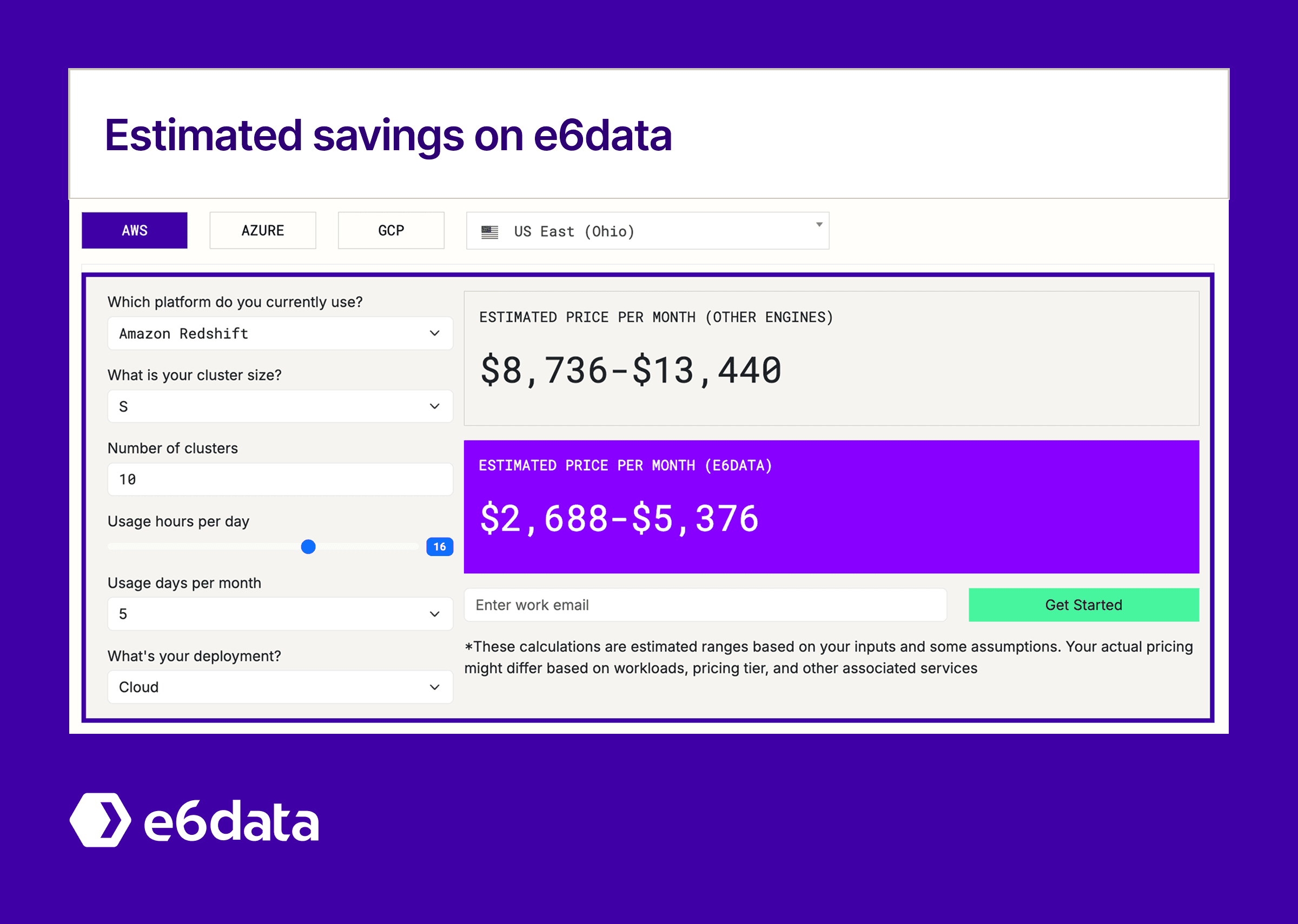
Key benefits of the e6data approach:

• Superior performance architecture: Decentralized vs. legacy centralized systems eliminates coordinator bottlenecks, delivers sub-second latency, and handles 1000+ concurrent users without SLA degradation through Kubernetes-native stateless services

• Zero vendor lock-in: Point directly at current lakehouse data with no movement, migrations, or architectural changes required. Full compatibility with existing governance, catalogs, and BI tools

• Predictable scaling & costs: Granular 1-vCPU increment scaling with per-vCPU billing eliminates cluster waste and surprise cost spikes. Instant performance with no cluster spin-up time or manual tuning overhead

Start a free trial of e6data and benchmark performance against your AWS Redshift workloads. Use our cost calculator to explore potential gains.