BigQuery's serverless architecture and automatic scaling deliver unmatched analytical performance, but that same flexibility can lead to unexpected cost spikes when teams optimize for speed without understanding the underlying slot-based pricing model. We've worked with dozens of data engineering teams running petabyte-scale analytics on BigQuery, and the pattern is consistent: costs often spiral when teams treat BigQuery as "pay-per-query" without considering slot utilization, data scanning patterns, and storage lifecycle management.
The reality? BigQuery's pricing complexity stems from its hybrid model: on-demand queries, reserved slots, storage tiers, and streaming inserts all follow different cost structures. Unlike traditional databases where you pay for fixed infrastructure, BigQuery charges for actual resource consumption, but optimizing that consumption requires understanding query execution patterns, data layout strategies, and workload classification.
This playbook focuses on practical optimizations that data engineering teams can implement immediately, organized by workload patterns that drive the highest costs. Each tactic includes runnable SQL configurations and BigQuery-specific monitoring queries, so you can start reducing costs without sacrificing the sub-second query performance your business users expect.
When does BigQuery spending become "high cost"?
Before diving into optimizations, it's crucial to establish what qualifies as "high cost" in BigQuery. These benchmarks help identify inefficient usage patterns:
Query cost per TB scanned · Threshold: >$6.00 per TB for routine analytics · Impact: Indicates poor partitioning, excessive SELECT *, or missing materialized views
Slot utilization efficiency · Threshold: >85% sustained usage or <20% average usage · Impact: Over-provisioning wastes money, under-provisioning creates queue delays
Storage growth rate · Threshold: >25% monthly without proportional query benefits · Impact: Poor lifecycle management or unnecessary data retention
Streaming insert costs · Threshold: >$0.02 per 1000 rows for real-time ingestion · Impact: Inefficient batch sizes or unnecessary streaming frequency
Data egress charges · Threshold: >$0.10/GB for cross-region transfers · Impact: Multi-region datasets with poor data locality
Query queue wait times · Threshold: >30 seconds average during peak hours · Impact: Under-provisioned slots or inefficient concurrent query patterns
Workload Taxonomy
BigQuery costs primarily spike when one of three usage patterns dominates your workload. Understanding which pattern drives your highest expenses is crucial for targeted optimization:
BI Dashboards - High-frequency analytical queries
Cost drivers: Repeated full-table scans, inefficient result caching, poor partitioning that doesn't match filter patterns, excessive slot allocation for peak concurrency, and materialized view maintenance overhead.
Optimization opportunities: Result caching eliminates duplicate computation, materialized views pre-aggregate frequent patterns, intelligent partitioning and clustering reduce scan volumes, and BI Engine acceleration delivers sub-second response times for small result sets.
Ad-hoc Analytics - Exploratory queries with unpredictable needs
Cost drivers: Full-table scans for hypothesis testing, lack of sampling strategies, inefficient JOIN operations, poor query complexity governance, and unnecessary precision in exploratory analysis that wastes compute resources.
Optimization opportunities: Intelligent data sampling reduces scan costs by 90%+ while maintaining statistical validity, approximate algorithms provide faster exploration, query complexity scoring prevents runaway costs, and federated queries minimize data movement expenses.
ETL/Streaming - High-volume data processing
Cost drivers: Inefficient batch loading patterns, streaming insert frequency that exceeds business requirements, poor compression and storage layout choices, unnecessary cross-region data replication, and suboptimal scheduling that creates slot contention.
Optimization opportunities: Optimized batch sizing and compression reduce storage and compute costs, streaming insert consolidation eliminates unnecessary micro-batching, data lifecycle policies automatically manage storage tiers, and intelligent scheduling spreads resource usage across lower-cost time windows.
BI Dashboards
Typical cost pitfalls: Oversized slot allocation for peak concurrency, repeated full-table scans for dashboard refreshes, and poor result caching strategies that miss obvious optimization opportunities.
1. Implement materialized views for dashboard acceleration to reduce query costs
A retail analytics team was refreshing executive dashboards against a large transactions table every 15 minutes. Each refresh scanned substantial amounts of data, consuming significant query costs daily for identical aggregations across product categories, regions, and time periods. Dashboard queries repeatedly aggregate the same dimensions, but BigQuery rescans and re-aggregates unless you persist the results in materialized views that incrementally update.
Fix: Materialized view pipeline for dashboard queries (an example scenario). This turns heavy queries that scanned billions of bytes into lightweight queries scanning just a few megabytes of pre-computed data.
-- Create base materialized view for daily sales aggregations
CREATE MATERIALIZED VIEW `analytics.daily_sales_summary`
PARTITION BY DATE(order_date)
CLUSTER BY region, category
AS
SELECT
    DATE(order_date) as order_date,
    region,
    category,
    COUNT(*) as order_count,
    SUM(amount) as total_revenue,
    AVG(amount) as avg_order_value,
    COUNT(DISTINCT customer_id) as unique_customers
FROM `sales.transactions`
WHERE order_date >= DATE_SUB(CURRENT_DATE(), INTERVAL 365 DAY)
GROUP BY 1, 2, 3;

-- Dashboard query now scans KB instead of TB
SELECT
    region,
    SUM(total_revenue) as revenue,
    SUM(order_count) as orders,
    AVG(avg_order_value) as avg_order_value
FROM `analytics.daily_sales_summary`
WHERE order_date >= DATE_SUB(CURRENT_DATE(), INTERVAL 30 DAY)
GROUP BY region
ORDER BY revenue DESC;

-- Monitor materialized view efficiency
SELECT
    table_name,
    last_refresh_time,
    refresh_watermark,
    size_bytes / 1e9 as size_gb
FROM `analytics.INFORMATION_SCHEMA.MATERIALIZED_VIEWS`
WHERE table_name = 'daily_sales_summary';
-- Create base materialized view for daily sales aggregations
CREATE MATERIALIZED VIEW `analytics.daily_sales_summary`
PARTITION BY DATE(order_date)
CLUSTER BY region, category
AS
SELECT
DATE(order_date) as order_date,
region,
category,
COUNT(*) as order_count,
SUM(amount) as total_revenue,
AVG(amount) as avg_order_value,
COUNT(DISTINCT customer_id) as unique_customers
FROM `sales.transactions`
WHERE order_date >= DATE_SUB(CURRENT_DATE(), INTERVAL 365 DAY)
GROUP BY 1, 2, 3;
-- Dashboard query now scans KB instead of TB
SELECT
region,
SUM(total_revenue) as revenue,
SUM(order_count) as orders,
AVG(avg_order_value) as avg_order_value
FROM `analytics.daily_sales_summary`
WHERE order_date >= DATE_SUB(CURRENT_DATE(), INTERVAL 30 DAY)
GROUP BY region
ORDER BY revenue DESC;
-- Monitor materialized view efficiency
SELECT
table_name,
last_refresh_time,
refresh_watermark,
size_bytes / 1e9 as size_gb
FROM `analytics.INFORMATION_SCHEMA.MATERIALIZED_VIEWS`
WHERE table_name = 'daily_sales_summary';-- Create base materialized view for daily sales aggregations
CREATE MATERIALIZED VIEW `analytics.daily_sales_summary`
PARTITION BY DATE(order_date)
CLUSTER BY region, category
AS
SELECT
DATE(order_date) as order_date,
region,
category,
COUNT(*) as order_count,
SUM(amount) as total_revenue,
AVG(amount) as avg_order_value,
COUNT(DISTINCT customer_id) as unique_customers
FROM `sales.transactions`
WHERE order_date >= DATE_SUB(CURRENT_DATE(), INTERVAL 365 DAY)
GROUP BY 1, 2, 3;
-- Dashboard query now scans KB instead of TB
SELECT
region,
SUM(total_revenue) as revenue,
SUM(order_count) as orders,
AVG(avg_order_value) as avg_order_value
FROM `analytics.daily_sales_summary`
WHERE order_date >= DATE_SUB(CURRENT_DATE(), INTERVAL 30 DAY)
GROUP BY region
ORDER BY revenue DESC;
-- Monitor materialized view efficiency
SELECT
table_name,
last_refresh_time,
refresh_watermark,
size_bytes / 1e9 as size_gb
FROM `analytics.INFORMATION_SCHEMA.MATERIALIZED_VIEWS`
WHERE table_name = 'daily_sales_summary';-- Create base materialized view for daily sales aggregations
CREATE MATERIALIZED VIEW `analytics.daily_sales_summary`
PARTITION BY DATE(order_date)
CLUSTER BY region, category
AS
SELECT
DATE(order_date) as order_date,
region,
category,
COUNT(*) as order_count,
SUM(amount) as total_revenue,
AVG(amount) as avg_order_value,
COUNT(DISTINCT customer_id) as unique_customers
FROM `sales.transactions`
WHERE order_date >= DATE_SUB(CURRENT_DATE(), INTERVAL 365 DAY)
GROUP BY 1, 2, 3;
-- Dashboard query now scans KB instead of TB
SELECT
region,
SUM(total_revenue) as revenue,
SUM(order_count) as orders,
AVG(avg_order_value) as avg_order_value
FROM `analytics.daily_sales_summary`
WHERE order_date >= DATE_SUB(CURRENT_DATE(), INTERVAL 30 DAY)
GROUP BY region
ORDER BY revenue DESC;
-- Monitor materialized view efficiency
SELECT
table_name,
last_refresh_time,
refresh_watermark,
size_bytes / 1e9 as size_gb
FROM `analytics.INFORMATION_SCHEMA.MATERIALIZED_VIEWS`
WHERE table_name = 'daily_sales_summary';Alternatives
Use scheduled queries to manually refresh aggregated tables with more control over timing and costs
Implement query result caching for static time periods to eliminate repeated computation
Consider BI Engine for sub-second acceleration of small result sets under 100GB
Use table snapshots for point-in-time dashboard views that don't require real-time data
Leverage e6data for variable dashboard workloads that benefit from per-vCPU autoscaling upto 1000 QPS+ instead of reserved slots
2. Optimize partitioning and clustering for dashboard filter patterns to improve query execution
A financial services dashboard was filtering a large customer events table by date ranges and account types, but the original partitioning strategy didn't match the dashboard filter patterns, forcing full partition scans across many date ranges.
Fix: Redesign partitioning strategy based on actual dashboard query patterns (an example scenario). In this case, partition by date (since every query uses a date range) and cluster by account_type (and perhaps event_type) so that queries which filter those fields will scan a much smaller subset of data.
-- Analyze existing query patterns to optimize partitioning
SELECT
    REGEXP_EXTRACT(query, r'WHERE.*?(?=GROUP|ORDER|LIMIT|$)') as where_patterns,
    COUNT(*) as frequency,
    AVG(total_bytes_billed / 1e12) as avg_tb_scanned
FROM `region-us.INFORMATION_SCHEMA.JOBS_BY_PROJECT`
WHERE creation_time >= TIMESTAMP_SUB(CURRENT_TIMESTAMP(), INTERVAL 30 DAY)
    AND query LIKE '%customer_events%'
    AND statement_type = 'SELECT'
GROUP BY where_patterns
ORDER BY frequency DESC
LIMIT 10;

-- Create optimally partitioned table
CREATE TABLE `analytics.customer_events_optimized` (
    event_date DATE,
    account_type STRING,
    customer_id STRING,
    event_type STRING,
    event_value NUMERIC
)
PARTITION BY event_date
CLUSTER BY account_type, event_type
OPTIONS(
    partition_expiration_days = 730,
    require_partition_filter = true
);

-- Migrate data with optimal layout
INSERT INTO `analytics.customer_events_optimized`
SELECT * FROM `analytics.customer_events`
WHERE event_date >= DATE_SUB(CURRENT_DATE(), INTERVAL 730 DAY);

-- Dashboard queries now skip irrelevant partitions
SELECT
    account_type,
    COUNT(*) as events,
    SUM(event_value) as total_value
FROM `analytics.customer_events_optimized`
WHERE event_date BETWEEN DATE_SUB(CURRENT_DATE(), INTERVAL 30 DAY) AND CURRENT_DATE()
    AND account_type IN ('premium', 'business')
GROUP BY account_type;
-- Analyze existing query patterns to optimize partitioning
SELECT
REGEXP_EXTRACT(query, r'WHERE.*?(?=GROUP|ORDER|LIMIT|$)') as where_patterns,
COUNT(*) as frequency,
AVG(total_bytes_billed / 1e12) as avg_tb_scanned
FROM `region-us.INFORMATION_SCHEMA.JOBS_BY_PROJECT`
WHERE creation_time >= TIMESTAMP_SUB(CURRENT_TIMESTAMP(), INTERVAL 30 DAY)
AND query LIKE '%customer_events%'
AND statement_type = 'SELECT'
GROUP BY where_patterns
ORDER BY frequency DESC
LIMIT 10;
-- Create optimally partitioned table
CREATE TABLE `analytics.customer_events_optimized` (
event_date DATE,
account_type STRING,
customer_id STRING,
event_type STRING,
event_value NUMERIC
)
PARTITION BY event_date
CLUSTER BY account_type, event_type
OPTIONS(
partition_expiration_days = 730,
require_partition_filter = true
);
-- Migrate data with optimal layout
INSERT INTO `analytics.customer_events_optimized`
SELECT * FROM `analytics.customer_events`
WHERE event_date >= DATE_SUB(CURRENT_DATE(), INTERVAL 730 DAY);
-- Dashboard queries now skip irrelevant partitions
SELECT
account_type,
COUNT(*) as events,
SUM(event_value) as total_value
FROM `analytics.customer_events_optimized`
WHERE event_date BETWEEN DATE_SUB(CURRENT_DATE(), INTERVAL 30 DAY) AND CURRENT_DATE()
AND account_type IN ('premium', 'business')
GROUP BY account_type;-- Analyze existing query patterns to optimize partitioning
SELECT
REGEXP_EXTRACT(query, r'WHERE.*?(?=GROUP|ORDER|LIMIT|$)') as where_patterns,
COUNT(*) as frequency,
AVG(total_bytes_billed / 1e12) as avg_tb_scanned
FROM `region-us.INFORMATION_SCHEMA.JOBS_BY_PROJECT`
WHERE creation_time >= TIMESTAMP_SUB(CURRENT_TIMESTAMP(), INTERVAL 30 DAY)
AND query LIKE '%customer_events%'
AND statement_type = 'SELECT'
GROUP BY where_patterns
ORDER BY frequency DESC
LIMIT 10;
-- Create optimally partitioned table
CREATE TABLE `analytics.customer_events_optimized` (
event_date DATE,
account_type STRING,
customer_id STRING,
event_type STRING,
event_value NUMERIC
)
PARTITION BY event_date
CLUSTER BY account_type, event_type
OPTIONS(
partition_expiration_days = 730,
require_partition_filter = true
);
-- Migrate data with optimal layout
INSERT INTO `analytics.customer_events_optimized`
SELECT * FROM `analytics.customer_events`
WHERE event_date >= DATE_SUB(CURRENT_DATE(), INTERVAL 730 DAY);
-- Dashboard queries now skip irrelevant partitions
SELECT
account_type,
COUNT(*) as events,
SUM(event_value) as total_value
FROM `analytics.customer_events_optimized`
WHERE event_date BETWEEN DATE_SUB(CURRENT_DATE(), INTERVAL 30 DAY) AND CURRENT_DATE()
AND account_type IN ('premium', 'business')
GROUP BY account_type;-- Analyze existing query patterns to optimize partitioning
SELECT
REGEXP_EXTRACT(query, r'WHERE.*?(?=GROUP|ORDER|LIMIT|$)') as where_patterns,
COUNT(*) as frequency,
AVG(total_bytes_billed / 1e12) as avg_tb_scanned
FROM `region-us.INFORMATION_SCHEMA.JOBS_BY_PROJECT`
WHERE creation_time >= TIMESTAMP_SUB(CURRENT_TIMESTAMP(), INTERVAL 30 DAY)
AND query LIKE '%customer_events%'
AND statement_type = 'SELECT'
GROUP BY where_patterns
ORDER BY frequency DESC
LIMIT 10;
-- Create optimally partitioned table
CREATE TABLE `analytics.customer_events_optimized` (
event_date DATE,
account_type STRING,
customer_id STRING,
event_type STRING,
event_value NUMERIC
)
PARTITION BY event_date
CLUSTER BY account_type, event_type
OPTIONS(
partition_expiration_days = 730,
require_partition_filter = true
);
-- Migrate data with optimal layout
INSERT INTO `analytics.customer_events_optimized`
SELECT * FROM `analytics.customer_events`
WHERE event_date >= DATE_SUB(CURRENT_DATE(), INTERVAL 730 DAY);
-- Dashboard queries now skip irrelevant partitions
SELECT
account_type,
COUNT(*) as events,
SUM(event_value) as total_value
FROM `analytics.customer_events_optimized`
WHERE event_date BETWEEN DATE_SUB(CURRENT_DATE(), INTERVAL 30 DAY) AND CURRENT_DATE()
AND account_type IN ('premium', 'business')
GROUP BY account_type;Alternatives
Use partition decorators for time-based queries to ensure partition pruning effectiveness
Implement time-unit column partitioning (hourly vs daily) based on dashboard refresh frequency
Consider range partitioning for non-date columns that have natural boundaries
Use clustering on multiple columns to optimize complex WHERE clauses
Apply query optimization techniques like predicate pushdown for nested and repeated fields
3. Implement intelligent result caching and query optimization to reduce duplicate computation
A marketing analytics platform ran the same complex cohort analysis queries many times daily across different dashboard users, with each query scanning large amounts of user behavior data and consuming significant costs per execution. There was no caching or reuse of results. Even though 90% of the logic was identical across these queries, BigQuery treated them as separate and scanned all the data each time. Small differences in the query SQL (like different literal values or slightly different SQL structure) meant the built-in cache wasn’t being hit.
Fix: Multi-level caching and query optimization strategy (an example scenario)
-- Enable query result caching and optimize cache hit rates
-- First, standardize query patterns to improve cache efficiency
CREATE OR REPLACE VIEW `analytics.cohort_analysis_base` AS
SELECT
    DATE_TRUNC(first_purchase_date, WEEK) as cohort_week,
    customer_id,
    DATE_DIFF(purchase_date, first_purchase_date, WEEK) as weeks_since_first_purchase,
    purchase_amount
FROM `sales.customer_purchases`
WHERE first_purchase_date >= DATE_SUB(CURRENT_DATE(), INTERVAL 52 WEEK);

-- Create cacheable cohort queries with consistent structure
WITH cohort_base AS (
    SELECT
        cohort_week,
        weeks_since_first_purchase,
        COUNT(DISTINCT customer_id) as customers,
        SUM(purchase_amount) as revenue
    FROM `analytics.cohort_analysis_base`
    WHERE cohort_week >= DATE_SUB(CURRENT_DATE(), INTERVAL 12 WEEK)
    GROUP BY 1, 2
),
cohort_sizes AS (
    SELECT
        cohort_week,
        COUNT(DISTINCT customer_id) as cohort_size
    FROM `analytics.cohort_analysis_base`
    WHERE weeks_since_first_purchase = 0
    GROUP BY 1
)
SELECT
    cb.cohort_week,
    cb.weeks_since_first_purchase,
    cb.customers,
    cb.revenue,
    cb.customers / cs.cohort_size as retention_rate
FROM cohort_base cb
JOIN cohort_sizes cs ON cb.cohort_week = cs.cohort_week
ORDER BY cb.cohort_week, cb.weeks_since_first_purchase;

-- Monitor cache hit rates and optimize queries for caching
SELECT
    job_id,
    query,
    cache_hit,
    total_bytes_billed / 1e9 as gb_billed,
    total_slot_ms / 1000 as slot_seconds
FROM `region-us.INFORMATION_SCHEMA.JOBS_BY_PROJECT`
WHERE creation_time >= TIMESTAMP_SUB(CURRENT_TIMESTAMP(), INTERVAL 1 DAY)
    AND statement_type = 'SELECT'
ORDER BY total_bytes_billed DESC;
-- Enable query result caching and optimize cache hit rates
-- First, standardize query patterns to improve cache efficiency
CREATE OR REPLACE VIEW `analytics.cohort_analysis_base` AS
SELECT
DATE_TRUNC(first_purchase_date, WEEK) as cohort_week,
customer_id,
DATE_DIFF(purchase_date, first_purchase_date, WEEK) as weeks_since_first_purchase,
purchase_amount
FROM `sales.customer_purchases`
WHERE first_purchase_date >= DATE_SUB(CURRENT_DATE(), INTERVAL 52 WEEK);
-- Create cacheable cohort queries with consistent structure
WITH cohort_base AS (
SELECT
cohort_week,
weeks_since_first_purchase,
COUNT(DISTINCT customer_id) as customers,
SUM(purchase_amount) as revenue
FROM `analytics.cohort_analysis_base`
WHERE cohort_week >= DATE_SUB(CURRENT_DATE(), INTERVAL 12 WEEK)
GROUP BY 1, 2
),
cohort_sizes AS (
SELECT
cohort_week,
COUNT(DISTINCT customer_id) as cohort_size
FROM `analytics.cohort_analysis_base`
WHERE weeks_since_first_purchase = 0
GROUP BY 1
)
SELECT
cb.cohort_week,
cb.weeks_since_first_purchase,
cb.customers,
cb.revenue,
cb.customers / cs.cohort_size as retention_rate
FROM cohort_base cb
JOIN cohort_sizes cs ON cb.cohort_week = cs.cohort_week
ORDER BY cb.cohort_week, cb.weeks_since_first_purchase;
-- Monitor cache hit rates and optimize queries for caching
SELECT
job_id,
query,
cache_hit,
total_bytes_billed / 1e9 as gb_billed,
total_slot_ms / 1000 as slot_seconds
FROM `region-us.INFORMATION_SCHEMA.JOBS_BY_PROJECT`
WHERE creation_time >= TIMESTAMP_SUB(CURRENT_TIMESTAMP(), INTERVAL 1 DAY)
AND statement_type = 'SELECT'
ORDER BY total_bytes_billed DESC;-- Enable query result caching and optimize cache hit rates
-- First, standardize query patterns to improve cache efficiency
CREATE OR REPLACE VIEW `analytics.cohort_analysis_base` AS
SELECT
DATE_TRUNC(first_purchase_date, WEEK) as cohort_week,
customer_id,
DATE_DIFF(purchase_date, first_purchase_date, WEEK) as weeks_since_first_purchase,
purchase_amount
FROM `sales.customer_purchases`
WHERE first_purchase_date >= DATE_SUB(CURRENT_DATE(), INTERVAL 52 WEEK);
-- Create cacheable cohort queries with consistent structure
WITH cohort_base AS (
SELECT
cohort_week,
weeks_since_first_purchase,
COUNT(DISTINCT customer_id) as customers,
SUM(purchase_amount) as revenue
FROM `analytics.cohort_analysis_base`
WHERE cohort_week >= DATE_SUB(CURRENT_DATE(), INTERVAL 12 WEEK)
GROUP BY 1, 2
),
cohort_sizes AS (
SELECT
cohort_week,
COUNT(DISTINCT customer_id) as cohort_size
FROM `analytics.cohort_analysis_base`
WHERE weeks_since_first_purchase = 0
GROUP BY 1
)
SELECT
cb.cohort_week,
cb.weeks_since_first_purchase,
cb.customers,
cb.revenue,
cb.customers / cs.cohort_size as retention_rate
FROM cohort_base cb
JOIN cohort_sizes cs ON cb.cohort_week = cs.cohort_week
ORDER BY cb.cohort_week, cb.weeks_since_first_purchase;
-- Monitor cache hit rates and optimize queries for caching
SELECT
job_id,
query,
cache_hit,
total_bytes_billed / 1e9 as gb_billed,
total_slot_ms / 1000 as slot_seconds
FROM `region-us.INFORMATION_SCHEMA.JOBS_BY_PROJECT`
WHERE creation_time >= TIMESTAMP_SUB(CURRENT_TIMESTAMP(), INTERVAL 1 DAY)
AND statement_type = 'SELECT'
ORDER BY total_bytes_billed DESC;-- Enable query result caching and optimize cache hit rates
-- First, standardize query patterns to improve cache efficiency
CREATE OR REPLACE VIEW `analytics.cohort_analysis_base` AS
SELECT
DATE_TRUNC(first_purchase_date, WEEK) as cohort_week,
customer_id,
DATE_DIFF(purchase_date, first_purchase_date, WEEK) as weeks_since_first_purchase,
purchase_amount
FROM `sales.customer_purchases`
WHERE first_purchase_date >= DATE_SUB(CURRENT_DATE(), INTERVAL 52 WEEK);
-- Create cacheable cohort queries with consistent structure
WITH cohort_base AS (
SELECT
cohort_week,
weeks_since_first_purchase,
COUNT(DISTINCT customer_id) as customers,
SUM(purchase_amount) as revenue
FROM `analytics.cohort_analysis_base`
WHERE cohort_week >= DATE_SUB(CURRENT_DATE(), INTERVAL 12 WEEK)
GROUP BY 1, 2
),
cohort_sizes AS (
SELECT
cohort_week,
COUNT(DISTINCT customer_id) as cohort_size
FROM `analytics.cohort_analysis_base`
WHERE weeks_since_first_purchase = 0
GROUP BY 1
)
SELECT
cb.cohort_week,
cb.weeks_since_first_purchase,
cb.customers,
cb.revenue,
cb.customers / cs.cohort_size as retention_rate
FROM cohort_base cb
JOIN cohort_sizes cs ON cb.cohort_week = cs.cohort_week
ORDER BY cb.cohort_week, cb.weeks_since_first_purchase;
-- Monitor cache hit rates and optimize queries for caching
SELECT
job_id,
query,
cache_hit,
total_bytes_billed / 1e9 as gb_billed,
total_slot_ms / 1000 as slot_seconds
FROM `region-us.INFORMATION_SCHEMA.JOBS_BY_PROJECT`
WHERE creation_time >= TIMESTAMP_SUB(CURRENT_TIMESTAMP(), INTERVAL 1 DAY)
AND statement_type = 'SELECT'
ORDER BY total_bytes_billed DESC;Alternatives
Use scheduled queries to pre-compute dashboard results and store them in dedicated tables
Create parameterized dashboard views that enable cache reuse across different filter combinations
Use BigQuery BI Engine for automatic caching of small result sets with sub-second access times
4. Configure slot autoscaling and workload isolation to reduce idle slot costs
A business intelligence team was paying for substantial reserved slots to handle peak dashboard loads during business hours, but utilization dropped significantly outside business hours and on weekends, wasting considerable monthly costs on idle capacity. If you allocate, say, 500 slots to guarantee low latency at peak, those slots cost the same 24/7. Without autoscaling or workload isolation, you either waste money or, if you try to go on-demand to save cost, you risk slowdowns at peak.
Fix: Implement autoscaling reservations with workload isolation (an example scenario)
-- Create separate reservations for different workload classes
-- Production dashboards: guaranteed capacity
CREATE RESERVATION `dashboard_production`
OPTIONS (
    slot_capacity = 500,
    location = 'US',
    edition = 'STANDARD'
);

-- Analytical workloads: flex slots for variable demand
CREATE RESERVATION `analytics_flex`
OPTIONS (
    slot_capacity = 100,
    location = 'US',
    edition = 'STANDARD',
    autoscale_max_slots = 1000
);

-- Assign projects to appropriate reservations
CREATE ASSIGNMENT `dashboard_assignment`
OPTIONS (
    assignee_type = 'PROJECT',
    assignee_id = 'dashboard-prod-project',
    job_type = 'QUERY',
    reservation = 'projects/your-project/locations/US/reservations/dashboard_production'
);

-- Monitor slot utilization and optimize reservation sizing
SELECT
    reservation_name,
    slot_capacity,
    APPROX_QUANTILES(total_slots, 4)[OFFSET(2)] as median_slots_used,
    AVG(total_slots) as avg_slots_used,
    MAX(total_slots) as peak_slots_used
FROM `region-us.INFORMATION_SCHEMA.RESERVATION_TIMELINE_BY_PROJECT`
WHERE start_time >= TIMESTAMP_SUB(CURRENT_TIMESTAMP(), INTERVAL 7 DAY)
GROUP BY reservation_name, slot_capacity
ORDER BY reservation_name;

-- Implement time-based slot scaling
CREATE OR REPLACE PROCEDURE `analytics.scale_slots`(target_slots INT64)
BEGIN
    EXECUTE IMMEDIATE FORMAT("""
        ALTER RESERVATION `analytics_flex`
        SET OPTIONS (slot_capacity = %d)
    """, target_slots);
END;
-- Create separate reservations for different workload classes
-- Production dashboards: guaranteed capacity
CREATE RESERVATION `dashboard_production`
OPTIONS (
slot_capacity = 500,
location = 'US',
edition = 'STANDARD'
);
-- Analytical workloads: flex slots for variable demand
CREATE RESERVATION `analytics_flex`
OPTIONS (
slot_capacity = 100,
location = 'US',
edition = 'STANDARD',
autoscale_max_slots = 1000
);
-- Assign projects to appropriate reservations
CREATE ASSIGNMENT `dashboard_assignment`
OPTIONS (
assignee_type = 'PROJECT',
assignee_id = 'dashboard-prod-project',
job_type = 'QUERY',
reservation = 'projects/your-project/locations/US/reservations/dashboard_production'
);
-- Monitor slot utilization and optimize reservation sizing
SELECT
reservation_name,
slot_capacity,
APPROX_QUANTILES(total_slots, 4)[OFFSET(2)] as median_slots_used,
AVG(total_slots) as avg_slots_used,
MAX(total_slots) as peak_slots_used
FROM `region-us.INFORMATION_SCHEMA.RESERVATION_TIMELINE_BY_PROJECT`
WHERE start_time >= TIMESTAMP_SUB(CURRENT_TIMESTAMP(), INTERVAL 7 DAY)
GROUP BY reservation_name, slot_capacity
ORDER BY reservation_name;
-- Implement time-based slot scaling
CREATE OR REPLACE PROCEDURE `analytics.scale_slots`(target_slots INT64)
BEGIN
EXECUTE IMMEDIATE FORMAT("""
ALTER RESERVATION `analytics_flex`
SET OPTIONS (slot_capacity = %d)
""", target_slots);
END;-- Create separate reservations for different workload classes
-- Production dashboards: guaranteed capacity
CREATE RESERVATION `dashboard_production`
OPTIONS (
slot_capacity = 500,
location = 'US',
edition = 'STANDARD'
);
-- Analytical workloads: flex slots for variable demand
CREATE RESERVATION `analytics_flex`
OPTIONS (
slot_capacity = 100,
location = 'US',
edition = 'STANDARD',
autoscale_max_slots = 1000
);
-- Assign projects to appropriate reservations
CREATE ASSIGNMENT `dashboard_assignment`
OPTIONS (
assignee_type = 'PROJECT',
assignee_id = 'dashboard-prod-project',
job_type = 'QUERY',
reservation = 'projects/your-project/locations/US/reservations/dashboard_production'
);
-- Monitor slot utilization and optimize reservation sizing
SELECT
reservation_name,
slot_capacity,
APPROX_QUANTILES(total_slots, 4)[OFFSET(2)] as median_slots_used,
AVG(total_slots) as avg_slots_used,
MAX(total_slots) as peak_slots_used
FROM `region-us.INFORMATION_SCHEMA.RESERVATION_TIMELINE_BY_PROJECT`
WHERE start_time >= TIMESTAMP_SUB(CURRENT_TIMESTAMP(), INTERVAL 7 DAY)
GROUP BY reservation_name, slot_capacity
ORDER BY reservation_name;
-- Implement time-based slot scaling
CREATE OR REPLACE PROCEDURE `analytics.scale_slots`(target_slots INT64)
BEGIN
EXECUTE IMMEDIATE FORMAT("""
ALTER RESERVATION `analytics_flex`
SET OPTIONS (slot_capacity = %d)
""", target_slots);
END;-- Create separate reservations for different workload classes
-- Production dashboards: guaranteed capacity
CREATE RESERVATION `dashboard_production`
OPTIONS (
slot_capacity = 500,
location = 'US',
edition = 'STANDARD'
);
-- Analytical workloads: flex slots for variable demand
CREATE RESERVATION `analytics_flex`
OPTIONS (
slot_capacity = 100,
location = 'US',
edition = 'STANDARD',
autoscale_max_slots = 1000
);
-- Assign projects to appropriate reservations
CREATE ASSIGNMENT `dashboard_assignment`
OPTIONS (
assignee_type = 'PROJECT',
assignee_id = 'dashboard-prod-project',
job_type = 'QUERY',
reservation = 'projects/your-project/locations/US/reservations/dashboard_production'
);
-- Monitor slot utilization and optimize reservation sizing
SELECT
reservation_name,
slot_capacity,
APPROX_QUANTILES(total_slots, 4)[OFFSET(2)] as median_slots_used,
AVG(total_slots) as avg_slots_used,
MAX(total_slots) as peak_slots_used
FROM `region-us.INFORMATION_SCHEMA.RESERVATION_TIMELINE_BY_PROJECT`
WHERE start_time >= TIMESTAMP_SUB(CURRENT_TIMESTAMP(), INTERVAL 7 DAY)
GROUP BY reservation_name, slot_capacity
ORDER BY reservation_name;
-- Implement time-based slot scaling
CREATE OR REPLACE PROCEDURE `analytics.scale_slots`(target_slots INT64)
BEGIN
EXECUTE IMMEDIATE FORMAT("""
ALTER RESERVATION `analytics_flex`
SET OPTIONS (slot_capacity = %d)
""", target_slots);
END;Alternatives
Use on-demand pricing for truly variable workloads instead of maintaining reservations
Implement query queuing and priority systems to better utilize available slot capacity
Schedule heavy analytical workloads during off-peak hours to reduce slot contention
Use BigQuery's job timeout settings to prevent runaway queries from consuming excessive slots
Consider hybrid deployment with e6data for complex workloads as it can autoscale up to 1000 QPS.
5. Leverage BI Engine for sub-second dashboard acceleration to improve user experience metrics
A customer support dashboard displaying real-time metrics was experiencing 5-15 second load times despite optimized queries, causing user frustration and reducing dashboard adoption across the support organization.
Fix: BI Engine configuration for accelerated dashboard performance (an example scenario)
-- Enable BI Engine for critical dashboard tables
ALTER TABLE `analytics.daily_sales_summary`
SET OPTIONS (
    max_staleness = INTERVAL '1' HOUR
);

-- Monitor BI Engine efficiency and cache hit rates
SELECT
    table_name,
    bi_engine_statistics.bi_engine_mode,
    bi_engine_statistics.bi_engine_reasons,
    total_logical_bytes / 1e9 as logical_gb,
    total_physical_bytes / 1e9 as physical_gb,
    bi_engine_statistics.bi_engine_acceleration.bi_engine_mode as acceleration_mode
FROM `analytics.INFORMATION_SCHEMA.TABLE_STORAGE_BY_PROJECT`
WHERE bi_engine_statistics.bi_engine_mode IS NOT NULL
    AND table_name IN ('daily_sales_summary', 'customer_metrics', 'support_tickets');

-- Optimize queries for BI Engine acceleration
-- Keep result sets under 100GB for optimal acceleration
SELECT
    support_agent,
    ticket_status,
    COUNT(*) as ticket_count,
    AVG(resolution_time_hours) as avg_resolution_time
FROM `support.tickets_summary`
WHERE created_date >= DATE_SUB(CURRENT_DATE(), INTERVAL 7 DAY)
    AND created_date <= CURRENT_DATE()
GROUP BY support_agent, ticket_status
HAVING ticket_count >= 5
ORDER BY ticket_count DESC
LIMIT 100;

-- Create BI Engine optimized views for common dashboard patterns
CREATE OR REPLACE VIEW `analytics.realtime_kpis` AS
SELECT
    DATE(event_timestamp) as event_date,
    EXTRACT(HOUR FROM event_timestamp) as event_hour,
    event_type,
    COUNT(*) as event_count,
    COUNT(DISTINCT user_id) as unique_users
FROM `events.user_interactions`
WHERE DATE(event_timestamp) >= DATE_SUB(CURRENT_DATE(), INTERVAL 30 DAY)
GROUP BY 1, 2, 3;
-- Enable BI Engine for critical dashboard tables
ALTER TABLE `analytics.daily_sales_summary`
SET OPTIONS (
max_staleness = INTERVAL '1' HOUR
);
-- Monitor BI Engine efficiency and cache hit rates
SELECT
table_name,
bi_engine_statistics.bi_engine_mode,
bi_engine_statistics.bi_engine_reasons,
total_logical_bytes / 1e9 as logical_gb,
total_physical_bytes / 1e9 as physical_gb,
bi_engine_statistics.bi_engine_acceleration.bi_engine_mode as acceleration_mode
FROM `analytics.INFORMATION_SCHEMA.TABLE_STORAGE_BY_PROJECT`
WHERE bi_engine_statistics.bi_engine_mode IS NOT NULL
AND table_name IN ('daily_sales_summary', 'customer_metrics', 'support_tickets');
-- Optimize queries for BI Engine acceleration
-- Keep result sets under 100GB for optimal acceleration
SELECT
support_agent,
ticket_status,
COUNT(*) as ticket_count,
AVG(resolution_time_hours) as avg_resolution_time
FROM `support.tickets_summary`
WHERE created_date >= DATE_SUB(CURRENT_DATE(), INTERVAL 7 DAY)
AND created_date <= CURRENT_DATE()
GROUP BY support_agent, ticket_status
HAVING ticket_count >= 5
ORDER BY ticket_count DESC
LIMIT 100;
-- Create BI Engine optimized views for common dashboard patterns
CREATE OR REPLACE VIEW `analytics.realtime_kpis` AS
SELECT
DATE(event_timestamp) as event_date,
EXTRACT(HOUR FROM event_timestamp) as event_hour,
event_type,
COUNT(*) as event_count,
COUNT(DISTINCT user_id) as unique_users
FROM `events.user_interactions`
WHERE DATE(event_timestamp) >= DATE_SUB(CURRENT_DATE(), INTERVAL 30 DAY)
GROUP BY 1, 2, 3;-- Enable BI Engine for critical dashboard tables
ALTER TABLE `analytics.daily_sales_summary`
SET OPTIONS (
max_staleness = INTERVAL '1' HOUR
);
-- Monitor BI Engine efficiency and cache hit rates
SELECT
table_name,
bi_engine_statistics.bi_engine_mode,
bi_engine_statistics.bi_engine_reasons,
total_logical_bytes / 1e9 as logical_gb,
total_physical_bytes / 1e9 as physical_gb,
bi_engine_statistics.bi_engine_acceleration.bi_engine_mode as acceleration_mode
FROM `analytics.INFORMATION_SCHEMA.TABLE_STORAGE_BY_PROJECT`
WHERE bi_engine_statistics.bi_engine_mode IS NOT NULL
AND table_name IN ('daily_sales_summary', 'customer_metrics', 'support_tickets');
-- Optimize queries for BI Engine acceleration
-- Keep result sets under 100GB for optimal acceleration
SELECT
support_agent,
ticket_status,
COUNT(*) as ticket_count,
AVG(resolution_time_hours) as avg_resolution_time
FROM `support.tickets_summary`
WHERE created_date >= DATE_SUB(CURRENT_DATE(), INTERVAL 7 DAY)
AND created_date <= CURRENT_DATE()
GROUP BY support_agent, ticket_status
HAVING ticket_count >= 5
ORDER BY ticket_count DESC
LIMIT 100;
-- Create BI Engine optimized views for common dashboard patterns
CREATE OR REPLACE VIEW `analytics.realtime_kpis` AS
SELECT
DATE(event_timestamp) as event_date,
EXTRACT(HOUR FROM event_timestamp) as event_hour,
event_type,
COUNT(*) as event_count,
COUNT(DISTINCT user_id) as unique_users
FROM `events.user_interactions`
WHERE DATE(event_timestamp) >= DATE_SUB(CURRENT_DATE(), INTERVAL 30 DAY)
GROUP BY 1, 2, 3;-- Enable BI Engine for critical dashboard tables
ALTER TABLE `analytics.daily_sales_summary`
SET OPTIONS (
max_staleness = INTERVAL '1' HOUR
);
-- Monitor BI Engine efficiency and cache hit rates
SELECT
table_name,
bi_engine_statistics.bi_engine_mode,
bi_engine_statistics.bi_engine_reasons,
total_logical_bytes / 1e9 as logical_gb,
total_physical_bytes / 1e9 as physical_gb,
bi_engine_statistics.bi_engine_acceleration.bi_engine_mode as acceleration_mode
FROM `analytics.INFORMATION_SCHEMA.TABLE_STORAGE_BY_PROJECT`
WHERE bi_engine_statistics.bi_engine_mode IS NOT NULL
AND table_name IN ('daily_sales_summary', 'customer_metrics', 'support_tickets');
-- Optimize queries for BI Engine acceleration
-- Keep result sets under 100GB for optimal acceleration
SELECT
support_agent,
ticket_status,
COUNT(*) as ticket_count,
AVG(resolution_time_hours) as avg_resolution_time
FROM `support.tickets_summary`
WHERE created_date >= DATE_SUB(CURRENT_DATE(), INTERVAL 7 DAY)
AND created_date <= CURRENT_DATE()
GROUP BY support_agent, ticket_status
HAVING ticket_count >= 5
ORDER BY ticket_count DESC
LIMIT 100;
-- Create BI Engine optimized views for common dashboard patterns
CREATE OR REPLACE VIEW `analytics.realtime_kpis` AS
SELECT
DATE(event_timestamp) as event_date,
EXTRACT(HOUR FROM event_timestamp) as event_hour,
event_type,
COUNT(*) as event_count,
COUNT(DISTINCT user_id) as unique_users
FROM `events.user_interactions`
WHERE DATE(event_timestamp) >= DATE_SUB(CURRENT_DATE(), INTERVAL 30 DAY)
GROUP BY 1, 2, 3;Alternatives
Use materialized views with frequent refresh schedules for near real-time performance
Implement application-level caching layers with Redis for sub-second response times
Create pre-aggregated summary tables that update incrementally throughout the day
Use streaming inserts with minute-level aggregations for real-time dashboard updates
Consider e6data's lakehouse query engine for consistent sub-second performance across variable workloads
Ad-hoc Analytics
Typical cost pitfalls: Full-table scans for exploratory queries, lack of intelligent sampling strategies, and poor query complexity governance that allows runaway costs.
1. Use TABLESAMPLE and intelligent sampling for exploration to reduce scan costs for hypothesis testing
A data science team was running full-table scans on their large customer behavior dataset to test simple hypotheses like "conversion rates by traffic source" or "seasonal patterns in user engagement." Each exploratory query was consuming substantial memory and generating significant costs per execution.
Full-table exploration wastes compute when representative samples provide equally valid statistical insights for hypothesis testing and pattern discovery.
Fix: Multi-level sampling strategy for cost-effective exploration (an example scenario)
-- Systematic sampling for representative analysis
SELECT
    traffic_source,
    COUNT(*) as total_users,
    COUNT(CASE WHEN converted = true THEN 1 END) as conversions,
    COUNT(CASE WHEN converted = true THEN 1 END) / COUNT(*) as conversion_rate
FROM `analytics.customer_journey` TABLESAMPLE SYSTEM (1 PERCENT)
WHERE visit_date >= DATE_SUB(CURRENT_DATE(), INTERVAL 90 DAY)
GROUP BY traffic_source
ORDER BY conversion_rate DESC;

-- Reservoir sampling for exact sample sizes regardless of table growth
SELECT
    device_type,
    session_duration_minutes,
    pages_viewed,
    purchase_amount
FROM `analytics.user_sessions` TABLESAMPLE RESERVOIR (10000 ROWS)
WHERE session_date >= DATE_SUB(CURRENT_DATE(), INTERVAL 30 DAY);

-- Stratified sampling for balanced representation across segments
WITH segment_samples AS (
    SELECT *, ROW_NUMBER() OVER (PARTITION BY user_segment ORDER BY RAND()) as rn
    FROM `analytics.user_profiles`
    WHERE last_active_date >= DATE_SUB(CURRENT_DATE(), INTERVAL 180 DAY)
)
SELECT
    user_segment,
    avg_monthly_spend,
    total_sessions,
    account_tenure_months
FROM segment_samples
WHERE rn <= 1000  -- 1000 users per segment
ORDER BY user_segment, avg_monthly_spend DESC;

-- Monitor sampling accuracy vs full table results
SELECT
    'full_table' as method,
    COUNT(*) as total_rows,
    AVG(session_duration) as avg_duration,
    STDDEV(session_duration) as duration_stddev
FROM `analytics.user_sessions`
WHERE session_date = CURRENT_DATE()

UNION ALL

SELECT
    'sampled_1pct' as method,
    COUNT(*) * 100 as extrapolated_total,  -- Scale up sample
    AVG(session_duration) as avg_duration,
    STDDEV(session_duration) as duration_stddev
FROM `analytics.user_sessions` TABLESAMPLE SYSTEM (1 PERCENT)
WHERE session_date = CURRENT_DATE();
-- Systematic sampling for representative analysis
SELECT
traffic_source,
COUNT(*) as total_users,
COUNT(CASE WHEN converted = true THEN 1 END) as conversions,
COUNT(CASE WHEN converted = true THEN 1 END) / COUNT(*) as conversion_rate
FROM `analytics.customer_journey` TABLESAMPLE SYSTEM (1 PERCENT)
WHERE visit_date >= DATE_SUB(CURRENT_DATE(), INTERVAL 90 DAY)
GROUP BY traffic_source
ORDER BY conversion_rate DESC;
-- Reservoir sampling for exact sample sizes regardless of table growth
SELECT
device_type,
session_duration_minutes,
pages_viewed,
purchase_amount
FROM `analytics.user_sessions` TABLESAMPLE RESERVOIR (10000 ROWS)
WHERE session_date >= DATE_SUB(CURRENT_DATE(), INTERVAL 30 DAY);
-- Stratified sampling for balanced representation across segments
WITH segment_samples AS (
SELECT *, ROW_NUMBER() OVER (PARTITION BY user_segment ORDER BY RAND()) as rn
FROM `analytics.user_profiles`
WHERE last_active_date >= DATE_SUB(CURRENT_DATE(), INTERVAL 180 DAY)
)
SELECT
user_segment,
avg_monthly_spend,
total_sessions,
account_tenure_months
FROM segment_samples
WHERE rn <= 1000 -- 1000 users per segment
ORDER BY user_segment, avg_monthly_spend DESC;
-- Monitor sampling accuracy vs full table results
SELECT
'full_table' as method,
COUNT(*) as total_rows,
AVG(session_duration) as avg_duration,
STDDEV(session_duration) as duration_stddev
FROM `analytics.user_sessions`
WHERE session_date = CURRENT_DATE()
UNION ALL
SELECT
'sampled_1pct' as method,
COUNT(*) * 100 as extrapolated_total, -- Scale up sample
AVG(session_duration) as avg_duration,
STDDEV(session_duration) as duration_stddev
FROM `analytics.user_sessions` TABLESAMPLE SYSTEM (1 PERCENT)
WHERE session_date = CURRENT_DATE();-- Systematic sampling for representative analysis
SELECT
traffic_source,
COUNT(*) as total_users,
COUNT(CASE WHEN converted = true THEN 1 END) as conversions,
COUNT(CASE WHEN converted = true THEN 1 END) / COUNT(*) as conversion_rate
FROM `analytics.customer_journey` TABLESAMPLE SYSTEM (1 PERCENT)
WHERE visit_date >= DATE_SUB(CURRENT_DATE(), INTERVAL 90 DAY)
GROUP BY traffic_source
ORDER BY conversion_rate DESC;
-- Reservoir sampling for exact sample sizes regardless of table growth
SELECT
device_type,
session_duration_minutes,
pages_viewed,
purchase_amount
FROM `analytics.user_sessions` TABLESAMPLE RESERVOIR (10000 ROWS)
WHERE session_date >= DATE_SUB(CURRENT_DATE(), INTERVAL 30 DAY);
-- Stratified sampling for balanced representation across segments
WITH segment_samples AS (
SELECT *, ROW_NUMBER() OVER (PARTITION BY user_segment ORDER BY RAND()) as rn
FROM `analytics.user_profiles`
WHERE last_active_date >= DATE_SUB(CURRENT_DATE(), INTERVAL 180 DAY)
)
SELECT
user_segment,
avg_monthly_spend,
total_sessions,
account_tenure_months
FROM segment_samples
WHERE rn <= 1000 -- 1000 users per segment
ORDER BY user_segment, avg_monthly_spend DESC;
-- Monitor sampling accuracy vs full table results
SELECT
'full_table' as method,
COUNT(*) as total_rows,
AVG(session_duration) as avg_duration,
STDDEV(session_duration) as duration_stddev
FROM `analytics.user_sessions`
WHERE session_date = CURRENT_DATE()
UNION ALL
SELECT
'sampled_1pct' as method,
COUNT(*) * 100 as extrapolated_total, -- Scale up sample
AVG(session_duration) as avg_duration,
STDDEV(session_duration) as duration_stddev
FROM `analytics.user_sessions` TABLESAMPLE SYSTEM (1 PERCENT)
WHERE session_date = CURRENT_DATE();-- Systematic sampling for representative analysis
SELECT
traffic_source,
COUNT(*) as total_users,
COUNT(CASE WHEN converted = true THEN 1 END) as conversions,
COUNT(CASE WHEN converted = true THEN 1 END) / COUNT(*) as conversion_rate
FROM `analytics.customer_journey` TABLESAMPLE SYSTEM (1 PERCENT)
WHERE visit_date >= DATE_SUB(CURRENT_DATE(), INTERVAL 90 DAY)
GROUP BY traffic_source
ORDER BY conversion_rate DESC;
-- Reservoir sampling for exact sample sizes regardless of table growth
SELECT
device_type,
session_duration_minutes,
pages_viewed,
purchase_amount
FROM `analytics.user_sessions` TABLESAMPLE RESERVOIR (10000 ROWS)
WHERE session_date >= DATE_SUB(CURRENT_DATE(), INTERVAL 30 DAY);
-- Stratified sampling for balanced representation across segments
WITH segment_samples AS (
SELECT *, ROW_NUMBER() OVER (PARTITION BY user_segment ORDER BY RAND()) as rn
FROM `analytics.user_profiles`
WHERE last_active_date >= DATE_SUB(CURRENT_DATE(), INTERVAL 180 DAY)
)
SELECT
user_segment,
avg_monthly_spend,
total_sessions,
account_tenure_months
FROM segment_samples
WHERE rn <= 1000 -- 1000 users per segment
ORDER BY user_segment, avg_monthly_spend DESC;
-- Monitor sampling accuracy vs full table results
SELECT
'full_table' as method,
COUNT(*) as total_rows,
AVG(session_duration) as avg_duration,
STDDEV(session_duration) as duration_stddev
FROM `analytics.user_sessions`
WHERE session_date = CURRENT_DATE()
UNION ALL
SELECT
'sampled_1pct' as method,
COUNT(*) * 100 as extrapolated_total, -- Scale up sample
AVG(session_duration) as avg_duration,
STDDEV(session_duration) as duration_stddev
FROM `analytics.user_sessions` TABLESAMPLE SYSTEM (1 PERCENT)
WHERE session_date = CURRENT_DATE();Alternatives
Create dedicated sample tables with automated refresh for repeated exploration patterns
Use approximate aggregate functions like HLL_COUNT.INIT for rapid cardinality estimation
Implement time-based sampling to focus analysis on recent, more relevant data periods
Build stratified sample views that maintain representation across key business dimension
2. Leverage approximate functions for faster statistical analysis to improve performance on large datasets
A marketing analytics team needed quick approximations of unique users, funnel conversion rates, and customer lifetime value across large datasets, but exact calculations were taking substantial time per query and consuming significant slot resources.
Exact computations on very large data (especially COUNT(DISTINCT), medians, 95th percentiles, top-k elements, etc.) require scanning and shuffling a lot of data. For example, counting distinct users over a big dataset can’t be easily broken down and usually triggers a large shuffle in BigQuery. Similarly, calculating precise percentiles can be heavy. Doing this frequently (say daily or ad-hoc) incurs big costs and might not be timely.
Fix: Approximate algorithm optimization for exploratory analytics (an example scenario)
-- Replace exact unique counts with HyperLogLog approximation
SELECT
    campaign_id,
    event_date,
    HLL_COUNT.MERGE(user_hll) as approx_unique_users,
    COUNT(*) as total_events,
    SUM(event_value) as total_value
FROM (
    SELECT
        campaign_id,
        event_date,
        HLL_COUNT.INIT(user_id) as user_hll,
        COUNT(*) as events,
        SUM(purchase_amount) as event_value
    FROM `marketing.campaign_events`
    WHERE event_date >= DATE_SUB(CURRENT_DATE(), INTERVAL 30 DAY)
    GROUP BY 1, 2
)
GROUP BY campaign_id, event_date
ORDER BY approx_unique_users DESC;

-- Use approximate quantiles for percentile analysis
SELECT
    product_category,
    APPROX_QUANTILES(price, 100)[OFFSET(25)] as p25_price,
    APPROX_QUANTILES(price, 100)[OFFSET(50)] as median_price,
    APPROX_QUANTILES(price, 100)[OFFSET(75)] as p75_price,
    APPROX_QUANTILES(price, 100)[OFFSET(95)] as p95_price
FROM `sales.product_purchases`
WHERE purchase_date >= DATE_SUB(CURRENT_DATE(), INTERVAL 90 DAY)
GROUP BY product_category;

-- Approximate top-K analysis for trending insights
SELECT
    APPROX_TOP_COUNT(search_query, 20) as top_searches,
    APPROX_TOP_SUM(search_query, clicks, 15) as top_searches_by_clicks
FROM `search.query_logs`
WHERE search_date = CURRENT_DATE();

-- Compare approximate vs exact for accuracy validation
WITH exact_results AS (
    SELECT
        COUNT(DISTINCT user_id) as exact_users,
        PERCENTILE_CONT(session_duration, 0.5) OVER() as exact_median
    FROM `analytics.sessions`
    WHERE DATE(session_start) = CURRENT_DATE()
),
approx_results AS (
    SELECT
        HLL_COUNT.INIT(user_id) as approx_users_hll,
        APPROX_QUANTILES(session_duration, 100)[OFFSET(50)] as approx_median
    FROM `analytics.sessions`
    WHERE DATE(session_start) = CURRENT_DATE()
)
SELECT
    HLL_COUNT.EXTRACT(approx_users_hll) as approx_users,
    exact_users,
    ABS(HLL_COUNT.EXTRACT(approx_users_hll) - exact_users) / exact_users as user_error_pct,
    approx_median,
    exact_median,
    ABS(approx_median - exact_median) / exact_median as median_error_pct
FROM exact_results, approx_results;
-- Replace exact unique counts with HyperLogLog approximation
SELECT
campaign_id,
event_date,
HLL_COUNT.MERGE(user_hll) as approx_unique_users,
COUNT(*) as total_events,
SUM(event_value) as total_value
FROM (
SELECT
campaign_id,
event_date,
HLL_COUNT.INIT(user_id) as user_hll,
COUNT(*) as events,
SUM(purchase_amount) as event_value
FROM `marketing.campaign_events`
WHERE event_date >= DATE_SUB(CURRENT_DATE(), INTERVAL 30 DAY)
GROUP BY 1, 2
)
GROUP BY campaign_id, event_date
ORDER BY approx_unique_users DESC;
-- Use approximate quantiles for percentile analysis
SELECT
product_category,
APPROX_QUANTILES(price, 100)[OFFSET(25)] as p25_price,
APPROX_QUANTILES(price, 100)[OFFSET(50)] as median_price,
APPROX_QUANTILES(price, 100)[OFFSET(75)] as p75_price,
APPROX_QUANTILES(price, 100)[OFFSET(95)] as p95_price
FROM `sales.product_purchases`
WHERE purchase_date >= DATE_SUB(CURRENT_DATE(), INTERVAL 90 DAY)
GROUP BY product_category;
-- Approximate top-K analysis for trending insights
SELECT
APPROX_TOP_COUNT(search_query, 20) as top_searches,
APPROX_TOP_SUM(search_query, clicks, 15) as top_searches_by_clicks
FROM `search.query_logs`
WHERE search_date = CURRENT_DATE();
-- Compare approximate vs exact for accuracy validation
WITH exact_results AS (
SELECT
COUNT(DISTINCT user_id) as exact_users,
PERCENTILE_CONT(session_duration, 0.5) OVER() as exact_median
FROM `analytics.sessions`
WHERE DATE(session_start) = CURRENT_DATE()
),
approx_results AS (
SELECT
HLL_COUNT.INIT(user_id) as approx_users_hll,
APPROX_QUANTILES(session_duration, 100)[OFFSET(50)] as approx_median
FROM `analytics.sessions`
WHERE DATE(session_start) = CURRENT_DATE()
)
SELECT
HLL_COUNT.EXTRACT(approx_users_hll) as approx_users,
exact_users,
ABS(HLL_COUNT.EXTRACT(approx_users_hll) - exact_users) / exact_users as user_error_pct,
approx_median,
exact_median,
ABS(approx_median - exact_median) / exact_median as median_error_pct
FROM exact_results, approx_results;-- Replace exact unique counts with HyperLogLog approximation
SELECT
campaign_id,
event_date,
HLL_COUNT.MERGE(user_hll) as approx_unique_users,
COUNT(*) as total_events,
SUM(event_value) as total_value
FROM (
SELECT
campaign_id,
event_date,
HLL_COUNT.INIT(user_id) as user_hll,
COUNT(*) as events,
SUM(purchase_amount) as event_value
FROM `marketing.campaign_events`
WHERE event_date >= DATE_SUB(CURRENT_DATE(), INTERVAL 30 DAY)
GROUP BY 1, 2
)
GROUP BY campaign_id, event_date
ORDER BY approx_unique_users DESC;
-- Use approximate quantiles for percentile analysis
SELECT
product_category,
APPROX_QUANTILES(price, 100)[OFFSET(25)] as p25_price,
APPROX_QUANTILES(price, 100)[OFFSET(50)] as median_price,
APPROX_QUANTILES(price, 100)[OFFSET(75)] as p75_price,
APPROX_QUANTILES(price, 100)[OFFSET(95)] as p95_price
FROM `sales.product_purchases`
WHERE purchase_date >= DATE_SUB(CURRENT_DATE(), INTERVAL 90 DAY)
GROUP BY product_category;
-- Approximate top-K analysis for trending insights
SELECT
APPROX_TOP_COUNT(search_query, 20) as top_searches,
APPROX_TOP_SUM(search_query, clicks, 15) as top_searches_by_clicks
FROM `search.query_logs`
WHERE search_date = CURRENT_DATE();
-- Compare approximate vs exact for accuracy validation
WITH exact_results AS (
SELECT
COUNT(DISTINCT user_id) as exact_users,
PERCENTILE_CONT(session_duration, 0.5) OVER() as exact_median
FROM `analytics.sessions`
WHERE DATE(session_start) = CURRENT_DATE()
),
approx_results AS (
SELECT
HLL_COUNT.INIT(user_id) as approx_users_hll,
APPROX_QUANTILES(session_duration, 100)[OFFSET(50)] as approx_median
FROM `analytics.sessions`
WHERE DATE(session_start) = CURRENT_DATE()
)
SELECT
HLL_COUNT.EXTRACT(approx_users_hll) as approx_users,
exact_users,
ABS(HLL_COUNT.EXTRACT(approx_users_hll) - exact_users) / exact_users as user_error_pct,
approx_median,
exact_median,
ABS(approx_median - exact_median) / exact_median as median_error_pct
FROM exact_results, approx_results;-- Replace exact unique counts with HyperLogLog approximation
SELECT
campaign_id,
event_date,
HLL_COUNT.MERGE(user_hll) as approx_unique_users,
COUNT(*) as total_events,
SUM(event_value) as total_value
FROM (
SELECT
campaign_id,
event_date,
HLL_COUNT.INIT(user_id) as user_hll,
COUNT(*) as events,
SUM(purchase_amount) as event_value
FROM `marketing.campaign_events`
WHERE event_date >= DATE_SUB(CURRENT_DATE(), INTERVAL 30 DAY)
GROUP BY 1, 2
)
GROUP BY campaign_id, event_date
ORDER BY approx_unique_users DESC;
-- Use approximate quantiles for percentile analysis
SELECT
product_category,
APPROX_QUANTILES(price, 100)[OFFSET(25)] as p25_price,
APPROX_QUANTILES(price, 100)[OFFSET(50)] as median_price,
APPROX_QUANTILES(price, 100)[OFFSET(75)] as p75_price,
APPROX_QUANTILES(price, 100)[OFFSET(95)] as p95_price
FROM `sales.product_purchases`
WHERE purchase_date >= DATE_SUB(CURRENT_DATE(), INTERVAL 90 DAY)
GROUP BY product_category;
-- Approximate top-K analysis for trending insights
SELECT
APPROX_TOP_COUNT(search_query, 20) as top_searches,
APPROX_TOP_SUM(search_query, clicks, 15) as top_searches_by_clicks
FROM `search.query_logs`
WHERE search_date = CURRENT_DATE();
-- Compare approximate vs exact for accuracy validation
WITH exact_results AS (
SELECT
COUNT(DISTINCT user_id) as exact_users,
PERCENTILE_CONT(session_duration, 0.5) OVER() as exact_median
FROM `analytics.sessions`
WHERE DATE(session_start) = CURRENT_DATE()
),
approx_results AS (
SELECT
HLL_COUNT.INIT(user_id) as approx_users_hll,
APPROX_QUANTILES(session_duration, 100)[OFFSET(50)] as approx_median
FROM `analytics.sessions`
WHERE DATE(session_start) = CURRENT_DATE()
)
SELECT
HLL_COUNT.EXTRACT(approx_users_hll) as approx_users,
exact_users,
ABS(HLL_COUNT.EXTRACT(approx_users_hll) - exact_users) / exact_users as user_error_pct,
approx_median,
exact_median,
ABS(approx_median - exact_median) / exact_median as median_error_pct
FROM exact_results, approx_results;Alternatives
Pre-compute exact statistics in scheduled batch jobs for frequently analyzed dimensions
Use BigQuery ML for approximate pattern recognition in large datasets
Implement hybrid approaches that use exact calculations for small result sets and approximations for large ones
Create approximate summary tables that update incrementally with streaming data
3. Implement query complexity scoring to prevent runaway costs and reduce expensive query incidents
A data science team had multiple expensive surprise bills when analysts accidentally created cartesian products or inefficient window functions across large tables, running for extended periods before manual intervention.
There was no proactive check on query complexity or cost before execution. BigQuery will let you run a 100TB join if you have the quota, and while you can set project-level quotas, sometimes these were broad. The team needed a way to catch obviously complex or potentially costly queries before they ran too long, or at least stop them quickly and inform the user.
Fix: Automated query complexity analysis and cost prevention (an example scenario)
-- Create query complexity analysis function
CREATE OR REPLACE FUNCTION `analytics.estimate_query_cost`(query_text STRING)
RETURNS STRUCT<
estimated_tb_scanned FLOAT64,
estimated_cost_usd FLOAT64,
complexity_score INT64,
risk_level STRING
>
LANGUAGE js AS """
var cost_per_tb = 5.0;
var complexity_score = 0;
var estimated_tb = 0.1;
if (query_text.includes('SELECT *')) complexity_score += 3;
if (query_text.includes('CROSS JOIN')) complexity_score += 5;
if (query_text.includes('WINDOW')) complexity_score += 2;
if ((query_text.match(/JOIN/g) || []).length > 3) complexity_score += 2;
estimated_tb = Math.pow(1.5, complexity_score) * 0.1;
var risk_level = complexity_score < 3 ? 'LOW' :
complexity_score < 6 ? 'MEDIUM' : 'HIGH';
return {
estimated_tb_scanned: estimated_tb,
estimated_cost_usd: estimated_tb * cost_per_tb,
complexity_score: complexity_score,
risk_level: risk_level
};
""";
-- Monitor and analyze expensive queries
CREATE OR REPLACE VIEW `analytics.query_cost_analysis` AS
WITH query_stats AS (
SELECT
job_id,
user_email,
query,
total_bytes_billed / 1e12 as tb_billed,
(total_bytes_billed / 1e12) * 5.0 as estimated_cost_usd,
total_slot_ms / 1000 as slot_seconds,
TIMESTAMP_DIFF(end_time, start_time, SECOND) as duration_seconds,
creation_time
FROM `region-us.INFORMATION_SCHEMA.JOBS_BY_PROJECT`
WHERE creation_time >= TIMESTAMP_SUB(CURRENT_TIMESTAMP(), INTERVAL 7 DAY)
AND state = 'DONE'
AND statement_type = 'SELECT'
)
SELECT
*,
analytics.estimate_query_cost(query) as complexity_analysis,
CASE
WHEN estimated_cost_usd > 50 THEN 'EXPENSIVE'
WHEN estimated_cost_usd > 10 THEN 'MODERATE'
ELSE 'CHEAP'
END as cost_category
FROM query_stats
WHERE tb_billed > 0.1 -- Focus on queries that scan >100GB
ORDER BY estimated_cost_usd DESC;
-- Create cost alerts and query governance
CREATE OR REPLACE PROCEDURE `analytics.check_query_cost_alerts`()
BEGIN
DECLARE alert_threshold FLOAT64 DEFAULT 25.0; -- $25 threshold
CREATE TEMP TABLE recent_expensive_queries AS
SELECT
job_id,
user_email,
estimated_cost_usd,
query,
creation_time
FROM `analytics.query_cost_analysis`
WHERE creation_time >= TIMESTAMP_SUB(CURRENT_TIMESTAMP(), INTERVAL 1 HOUR)
AND estimated_cost_usd > alert_threshold;
-- Alert logic would integrate with notification systems
SELECT
CONCAT('COST ALERT: Query ', job_id, ' by ', user_email,
' cost $', ROUND(estimated_cost_usd, 2)) as alert_message,
query,
creation_time
FROM recent_expensive_queries;
END;-- Create query complexity analysis function
CREATE OR REPLACE FUNCTION `analytics.estimate_query_cost`(query_text STRING)
RETURNS STRUCT<
estimated_tb_scanned FLOAT64,
estimated_cost_usd FLOAT64,
complexity_score INT64,
risk_level STRING
>
LANGUAGE js AS """
var cost_per_tb = 5.0;
var complexity_score = 0;
var estimated_tb = 0.1;
if (query_text.includes('SELECT *')) complexity_score += 3;
if (query_text.includes('CROSS JOIN')) complexity_score += 5;
if (query_text.includes('WINDOW')) complexity_score += 2;
if ((query_text.match(/JOIN/g) || []).length > 3) complexity_score += 2;
estimated_tb = Math.pow(1.5, complexity_score) * 0.1;
var risk_level = complexity_score < 3 ? 'LOW' :
complexity_score < 6 ? 'MEDIUM' : 'HIGH';
return {
estimated_tb_scanned: estimated_tb,
estimated_cost_usd: estimated_tb * cost_per_tb,
complexity_score: complexity_score,
risk_level: risk_level
};
""";
-- Monitor and analyze expensive queries
CREATE OR REPLACE VIEW `analytics.query_cost_analysis` AS
WITH query_stats AS (
SELECT
job_id,
user_email,
query,
total_bytes_billed / 1e12 as tb_billed,
(total_bytes_billed / 1e12) * 5.0 as estimated_cost_usd,
total_slot_ms / 1000 as slot_seconds,
TIMESTAMP_DIFF(end_time, start_time, SECOND) as duration_seconds,
creation_time
FROM `region-us.INFORMATION_SCHEMA.JOBS_BY_PROJECT`
WHERE creation_time >= TIMESTAMP_SUB(CURRENT_TIMESTAMP(), INTERVAL 7 DAY)
AND state = 'DONE'
AND statement_type = 'SELECT'
)
SELECT
*,
analytics.estimate_query_cost(query) as complexity_analysis,
CASE
WHEN estimated_cost_usd > 50 THEN 'EXPENSIVE'
WHEN estimated_cost_usd > 10 THEN 'MODERATE'
ELSE 'CHEAP'
END as cost_category
FROM query_stats
WHERE tb_billed > 0.1 -- Focus on queries that scan >100GB
ORDER BY estimated_cost_usd DESC;
-- Create cost alerts and query governance
CREATE OR REPLACE PROCEDURE `analytics.check_query_cost_alerts`()
BEGIN
DECLARE alert_threshold FLOAT64 DEFAULT 25.0; -- $25 threshold
CREATE TEMP TABLE recent_expensive_queries AS
SELECT
job_id,
user_email,
estimated_cost_usd,
query,
creation_time
FROM `analytics.query_cost_analysis`
WHERE creation_time >= TIMESTAMP_SUB(CURRENT_TIMESTAMP(), INTERVAL 1 HOUR)
AND estimated_cost_usd > alert_threshold;
-- Alert logic would integrate with notification systems
SELECT
CONCAT('COST ALERT: Query ', job_id, ' by ', user_email,
' cost $', ROUND(estimated_cost_usd, 2)) as alert_message,
query,
creation_time
FROM recent_expensive_queries;
END;-- Create query complexity analysis function
CREATE OR REPLACE FUNCTION `analytics.estimate_query_cost`(query_text STRING)
RETURNS STRUCT<
estimated_tb_scanned FLOAT64,
estimated_cost_usd FLOAT64,
complexity_score INT64,
risk_level STRING
>
LANGUAGE js AS """
var cost_per_tb = 5.0;
var complexity_score = 0;
var estimated_tb = 0.1;
if (query_text.includes('SELECT *')) complexity_score += 3;
if (query_text.includes('CROSS JOIN')) complexity_score += 5;
if (query_text.includes('WINDOW')) complexity_score += 2;
if ((query_text.match(/JOIN/g) || []).length > 3) complexity_score += 2;
estimated_tb = Math.pow(1.5, complexity_score) * 0.1;
var risk_level = complexity_score < 3 ? 'LOW' :
complexity_score < 6 ? 'MEDIUM' : 'HIGH';
return {
estimated_tb_scanned: estimated_tb,
estimated_cost_usd: estimated_tb * cost_per_tb,
complexity_score: complexity_score,
risk_level: risk_level
};
""";
-- Monitor and analyze expensive queries
CREATE OR REPLACE VIEW `analytics.query_cost_analysis` AS
WITH query_stats AS (
SELECT
job_id,
user_email,
query,
total_bytes_billed / 1e12 as tb_billed,
(total_bytes_billed / 1e12) * 5.0 as estimated_cost_usd,
total_slot_ms / 1000 as slot_seconds,
TIMESTAMP_DIFF(end_time, start_time, SECOND) as duration_seconds,
creation_time
FROM `region-us.INFORMATION_SCHEMA.JOBS_BY_PROJECT`
WHERE creation_time >= TIMESTAMP_SUB(CURRENT_TIMESTAMP(), INTERVAL 7 DAY)
AND state = 'DONE'
AND statement_type = 'SELECT'
)
SELECT
*,
analytics.estimate_query_cost(query) as complexity_analysis,
CASE
WHEN estimated_cost_usd > 50 THEN 'EXPENSIVE'
WHEN estimated_cost_usd > 10 THEN 'MODERATE'
ELSE 'CHEAP'
END as cost_category
FROM query_stats
WHERE tb_billed > 0.1 -- Focus on queries that scan >100GB
ORDER BY estimated_cost_usd DESC;
-- Create cost alerts and query governance
CREATE OR REPLACE PROCEDURE `analytics.check_query_cost_alerts`()
BEGIN
DECLARE alert_threshold FLOAT64 DEFAULT 25.0; -- $25 threshold
CREATE TEMP TABLE recent_expensive_queries AS
SELECT
job_id,
user_email,
estimated_cost_usd,
query,
creation_time
FROM `analytics.query_cost_analysis`
WHERE creation_time >= TIMESTAMP_SUB(CURRENT_TIMESTAMP(), INTERVAL 1 HOUR)
AND estimated_cost_usd > alert_threshold;
-- Alert logic would integrate with notification systems
SELECT
CONCAT('COST ALERT: Query ', job_id, ' by ', user_email,
' cost $', ROUND(estimated_cost_usd, 2)) as alert_message,
query,
creation_time
FROM recent_expensive_queries;
END;-- Create query complexity analysis function
CREATE OR REPLACE FUNCTION `analytics.estimate_query_cost`(query_text STRING)
RETURNS STRUCT<
estimated_tb_scanned FLOAT64,
estimated_cost_usd FLOAT64,
complexity_score INT64,
risk_level STRING
>
LANGUAGE js AS """
var cost_per_tb = 5.0;
var complexity_score = 0;
var estimated_tb = 0.1;
if (query_text.includes('SELECT *')) complexity_score += 3;
if (query_text.includes('CROSS JOIN')) complexity_score += 5;
if (query_text.includes('WINDOW')) complexity_score += 2;
if ((query_text.match(/JOIN/g) || []).length > 3) complexity_score += 2;
estimated_tb = Math.pow(1.5, complexity_score) * 0.1;
var risk_level = complexity_score < 3 ? 'LOW' :
complexity_score < 6 ? 'MEDIUM' : 'HIGH';
return {
estimated_tb_scanned: estimated_tb,
estimated_cost_usd: estimated_tb * cost_per_tb,
complexity_score: complexity_score,
risk_level: risk_level
};
""";
-- Monitor and analyze expensive queries
CREATE OR REPLACE VIEW `analytics.query_cost_analysis` AS
WITH query_stats AS (
SELECT
job_id,
user_email,
query,
total_bytes_billed / 1e12 as tb_billed,
(total_bytes_billed / 1e12) * 5.0 as estimated_cost_usd,
total_slot_ms / 1000 as slot_seconds,
TIMESTAMP_DIFF(end_time, start_time, SECOND) as duration_seconds,
creation_time
FROM `region-us.INFORMATION_SCHEMA.JOBS_BY_PROJECT`
WHERE creation_time >= TIMESTAMP_SUB(CURRENT_TIMESTAMP(), INTERVAL 7 DAY)
AND state = 'DONE'
AND statement_type = 'SELECT'
)
SELECT
*,
analytics.estimate_query_cost(query) as complexity_analysis,
CASE
WHEN estimated_cost_usd > 50 THEN 'EXPENSIVE'
WHEN estimated_cost_usd > 10 THEN 'MODERATE'
ELSE 'CHEAP'
END as cost_category
FROM query_stats
WHERE tb_billed > 0.1 -- Focus on queries that scan >100GB
ORDER BY estimated_cost_usd DESC;
-- Create cost alerts and query governance
CREATE OR REPLACE PROCEDURE `analytics.check_query_cost_alerts`()
BEGIN
DECLARE alert_threshold FLOAT64 DEFAULT 25.0; -- $25 threshold
CREATE TEMP TABLE recent_expensive_queries AS
SELECT
job_id,
user_email,
estimated_cost_usd,
query,
creation_time
FROM `analytics.query_cost_analysis`
WHERE creation_time >= TIMESTAMP_SUB(CURRENT_TIMESTAMP(), INTERVAL 1 HOUR)
AND estimated_cost_usd > alert_threshold;
-- Alert logic would integrate with notification systems
SELECT
CONCAT('COST ALERT: Query ', job_id, ' by ', user_email,
' cost $', ROUND(estimated_cost_usd, 2)) as alert_message,
query,
creation_time
FROM recent_expensive_queries;
END;Alternatives
Implement query approval workflows for complex queries above cost thresholds
Use BigQuery's maximum bytes billed setting to hard-cap individual query costs
Create query templates and best practice guidelines for common analytical patterns
Set up automated query optimization suggestions based on execution patterns
Use e6data's built-in cost controls and automatic query optimization for variable workloads
4. Optimize JOIN strategies and query structure for large analytical queries to reduce execution time
A business intelligence team was running multi-table analytical queries across large fact tables and dimension tables, consuming substantial memory per query and taking considerable time to complete.
Joining a huge fact table with multiple dimensions at full granularity can be very expensive if you only ultimately needed an aggregated result. Similarly, if you join two huge tables and then filter, it’s often better to filter first or pre-aggregate to reduce data. The default join order or type might not be optimal for every scenario (though the query planner does a decent job).
Fix: Advanced JOIN optimization and query restructuring (example scenario)
-- Optimize join order and use appropriate join types
-- First, analyze table cardinalities to inform join strategy
SELECT
    table_name,
    row_count,
    size_bytes / 1e9 as size_gb,
    partitioning_type,
    clustering_fields
FROM `analytics.INFORMATION_SCHEMA.TABLE_STORAGE_BY_PROJECT`
WHERE table_name IN ('customer_orders', 'products', 'customers', 'stores')
ORDER BY row_count DESC;

-- Use broadcast joins for small dimension tables
SELECT
    o.order_id,
    c.customer_segment,
    p.product_category,
    s.store_region,
    o.order_amount
FROM `sales.customer_orders` o
LEFT JOIN `reference.customers` c ON o.customer_id = c.customer_id
LEFT JOIN `reference.products` p ON o.product_id = p.product_id
LEFT JOIN `reference.stores` s ON o.store_id = s.store_id
WHERE o.order_date >= DATE_SUB(CURRENT_DATE(), INTERVAL 30 DAY);

-- Pre-aggregate before expensive joins
WITH daily_sales AS (
    SELECT
        order_date,
        customer_id,
        store_id,
        COUNT(*) as order_count,
        SUM(order_amount) as daily_amount,
        AVG(order_amount) as avg_order_value
    FROM `sales.customer_orders`
    WHERE order_date >= DATE_SUB(CURRENT_DATE(), INTERVAL 90 DAY)
    GROUP BY 1, 2, 3
),
customer_metrics AS (
    SELECT
        customer_id,
        COUNT(DISTINCT order_date) as active_days,
        SUM(daily_amount) as total_spent,
        AVG(avg_order_value) as avg_order_value
    FROM daily_sales
    GROUP BY customer_id
)
SELECT
    cm.customer_id,
    c.customer_segment,
    cm.active_days,
    cm.total_spent,
    cm.avg_order_value
FROM customer_metrics cm
JOIN `reference.customers` c ON cm.customer_id = c.customer_id
WHERE cm.total_spent >= 1000
ORDER BY cm.total_spent DESC;

-- Use window functions efficiently to avoid self-joins
SELECT
    customer_id,
    order_date,
    order_amount,
    -- Calculate running totals and rankings in single pass
    SUM(order_amount) OVER (
        PARTITION BY customer_id
        ORDER BY order_date
        ROWS UNBOUNDED PRECEDING
    ) as running_total,
    ROW_NUMBER() OVER (
        PARTITION BY customer_id
        ORDER BY order_amount DESC
    ) as amount_rank,
    LAG(order_amount) OVER (
        PARTITION BY customer_id
        ORDER BY order_date
    ) as previous_order_amount
FROM `sales.customer_orders`
WHERE order_date >= DATE_SUB(CURRENT_DATE(), INTERVAL 365 DAY)
QUALIFY amount_rank <= 5;  -- Top 5 orders per customer

-- Monitor join performance and optimization opportunities
SELECT
    job_id,
    query,
    total_slot_ms / 1000 as slot_seconds,
    max_slots_utilized,
    total_bytes_processed / 1e9 as gb_processed,
    TIMESTAMP_DIFF(end_time, start_time, SECOND) as duration_seconds
FROM `region-us.INFORMATION_SCHEMA.JOBS_BY_PROJECT`
WHERE creation_time >= TIMESTAMP_SUB(CURRENT_TIMESTAMP(), INTERVAL 1 DAY)
    AND query LIKE '%JOIN%'
    AND total_slot_ms > 60000  -- Queries using >60 slot-seconds
ORDER BY total_slot_ms DESC;
-- Optimize join order and use appropriate join types
-- First, analyze table cardinalities to inform join strategy
SELECT
table_name,
row_count,
size_bytes / 1e9 as size_gb,
partitioning_type,
clustering_fields
FROM `analytics.INFORMATION_SCHEMA.TABLE_STORAGE_BY_PROJECT`
WHERE table_name IN ('customer_orders', 'products', 'customers', 'stores')
ORDER BY row_count DESC;
-- Use broadcast joins for small dimension tables
SELECT
o.order_id,
c.customer_segment,
p.product_category,
s.store_region,
o.order_amount
FROM `sales.customer_orders` o
LEFT JOIN `reference.customers` c ON o.customer_id = c.customer_id
LEFT JOIN `reference.products` p ON o.product_id = p.product_id
LEFT JOIN `reference.stores` s ON o.store_id = s.store_id
WHERE o.order_date >= DATE_SUB(CURRENT_DATE(), INTERVAL 30 DAY);
-- Pre-aggregate before expensive joins
WITH daily_sales AS (
SELECT
order_date,
customer_id,
store_id,
COUNT(*) as order_count,
SUM(order_amount) as daily_amount,
AVG(order_amount) as avg_order_value
FROM `sales.customer_orders`
WHERE order_date >= DATE_SUB(CURRENT_DATE(), INTERVAL 90 DAY)
GROUP BY 1, 2, 3
),
customer_metrics AS (
SELECT
customer_id,
COUNT(DISTINCT order_date) as active_days,
SUM(daily_amount) as total_spent,
AVG(avg_order_value) as avg_order_value
FROM daily_sales
GROUP BY customer_id
)
SELECT
cm.customer_id,
c.customer_segment,
cm.active_days,
cm.total_spent,
cm.avg_order_value
FROM customer_metrics cm
JOIN `reference.customers` c ON cm.customer_id = c.customer_id
WHERE cm.total_spent >= 1000
ORDER BY cm.total_spent DESC;
-- Use window functions efficiently to avoid self-joins
SELECT
customer_id,
order_date,
order_amount,
-- Calculate running totals and rankings in single pass
SUM(order_amount) OVER (
PARTITION BY customer_id
ORDER BY order_date
ROWS UNBOUNDED PRECEDING
) as running_total,
ROW_NUMBER() OVER (
PARTITION BY customer_id
ORDER BY order_amount DESC
) as amount_rank,
LAG(order_amount) OVER (
PARTITION BY customer_id
ORDER BY order_date
) as previous_order_amount
FROM `sales.customer_orders`
WHERE order_date >= DATE_SUB(CURRENT_DATE(), INTERVAL 365 DAY)
QUALIFY amount_rank <= 5; -- Top 5 orders per customer
-- Monitor join performance and optimization opportunities
SELECT
job_id,
query,
total_slot_ms / 1000 as slot_seconds,
max_slots_utilized,
total_bytes_processed / 1e9 as gb_processed,
TIMESTAMP_DIFF(end_time, start_time, SECOND) as duration_seconds
FROM `region-us.INFORMATION_SCHEMA.JOBS_BY_PROJECT`
WHERE creation_time >= TIMESTAMP_SUB(CURRENT_TIMESTAMP(), INTERVAL 1 DAY)
AND query LIKE '%JOIN%'
AND total_slot_ms > 60000 -- Queries using >60 slot-seconds
ORDER BY total_slot_ms DESC;-- Optimize join order and use appropriate join types
-- First, analyze table cardinalities to inform join strategy
SELECT
table_name,
row_count,
size_bytes / 1e9 as size_gb,
partitioning_type,
clustering_fields
FROM `analytics.INFORMATION_SCHEMA.TABLE_STORAGE_BY_PROJECT`
WHERE table_name IN ('customer_orders', 'products', 'customers', 'stores')
ORDER BY row_count DESC;
-- Use broadcast joins for small dimension tables
SELECT
o.order_id,
c.customer_segment,
p.product_category,
s.store_region,
o.order_amount
FROM `sales.customer_orders` o
LEFT JOIN `reference.customers` c ON o.customer_id = c.customer_id
LEFT JOIN `reference.products` p ON o.product_id = p.product_id
LEFT JOIN `reference.stores` s ON o.store_id = s.store_id
WHERE o.order_date >= DATE_SUB(CURRENT_DATE(), INTERVAL 30 DAY);
-- Pre-aggregate before expensive joins
WITH daily_sales AS (
SELECT
order_date,
customer_id,
store_id,
COUNT(*) as order_count,
SUM(order_amount) as daily_amount,
AVG(order_amount) as avg_order_value
FROM `sales.customer_orders`
WHERE order_date >= DATE_SUB(CURRENT_DATE(), INTERVAL 90 DAY)
GROUP BY 1, 2, 3
),
customer_metrics AS (
SELECT
customer_id,
COUNT(DISTINCT order_date) as active_days,
SUM(daily_amount) as total_spent,
AVG(avg_order_value) as avg_order_value
FROM daily_sales
GROUP BY customer_id
)
SELECT
cm.customer_id,
c.customer_segment,
cm.active_days,
cm.total_spent,
cm.avg_order_value
FROM customer_metrics cm
JOIN `reference.customers` c ON cm.customer_id = c.customer_id
WHERE cm.total_spent >= 1000
ORDER BY cm.total_spent DESC;
-- Use window functions efficiently to avoid self-joins
SELECT
customer_id,
order_date,
order_amount,
-- Calculate running totals and rankings in single pass
SUM(order_amount) OVER (
PARTITION BY customer_id
ORDER BY order_date
ROWS UNBOUNDED PRECEDING
) as running_total,
ROW_NUMBER() OVER (
PARTITION BY customer_id
ORDER BY order_amount DESC
) as amount_rank,
LAG(order_amount) OVER (
PARTITION BY customer_id
ORDER BY order_date
) as previous_order_amount
FROM `sales.customer_orders`
WHERE order_date >= DATE_SUB(CURRENT_DATE(), INTERVAL 365 DAY)
QUALIFY amount_rank <= 5; -- Top 5 orders per customer
-- Monitor join performance and optimization opportunities
SELECT
job_id,
query,
total_slot_ms / 1000 as slot_seconds,
max_slots_utilized,
total_bytes_processed / 1e9 as gb_processed,
TIMESTAMP_DIFF(end_time, start_time, SECOND) as duration_seconds
FROM `region-us.INFORMATION_SCHEMA.JOBS_BY_PROJECT`
WHERE creation_time >= TIMESTAMP_SUB(CURRENT_TIMESTAMP(), INTERVAL 1 DAY)
AND query LIKE '%JOIN%'
AND total_slot_ms > 60000 -- Queries using >60 slot-seconds
ORDER BY total_slot_ms DESC;-- Optimize join order and use appropriate join types
-- First, analyze table cardinalities to inform join strategy
SELECT
table_name,
row_count,
size_bytes / 1e9 as size_gb,
partitioning_type,
clustering_fields
FROM `analytics.INFORMATION_SCHEMA.TABLE_STORAGE_BY_PROJECT`
WHERE table_name IN ('customer_orders', 'products', 'customers', 'stores')
ORDER BY row_count DESC;
-- Use broadcast joins for small dimension tables
SELECT
o.order_id,
c.customer_segment,
p.product_category,
s.store_region,
o.order_amount
FROM `sales.customer_orders` o
LEFT JOIN `reference.customers` c ON o.customer_id = c.customer_id
LEFT JOIN `reference.products` p ON o.product_id = p.product_id
LEFT JOIN `reference.stores` s ON o.store_id = s.store_id
WHERE o.order_date >= DATE_SUB(CURRENT_DATE(), INTERVAL 30 DAY);
-- Pre-aggregate before expensive joins
WITH daily_sales AS (
SELECT
order_date,
customer_id,
store_id,
COUNT(*) as order_count,
SUM(order_amount) as daily_amount,
AVG(order_amount) as avg_order_value
FROM `sales.customer_orders`
WHERE order_date >= DATE_SUB(CURRENT_DATE(), INTERVAL 90 DAY)
GROUP BY 1, 2, 3
),
customer_metrics AS (
SELECT
customer_id,
COUNT(DISTINCT order_date) as active_days,
SUM(daily_amount) as total_spent,
AVG(avg_order_value) as avg_order_value
FROM daily_sales
GROUP BY customer_id
)
SELECT
cm.customer_id,
c.customer_segment,
cm.active_days,
cm.total_spent,
cm.avg_order_value
FROM customer_metrics cm
JOIN `reference.customers` c ON cm.customer_id = c.customer_id
WHERE cm.total_spent >= 1000
ORDER BY cm.total_spent DESC;
-- Use window functions efficiently to avoid self-joins
SELECT
customer_id,
order_date,
order_amount,
-- Calculate running totals and rankings in single pass
SUM(order_amount) OVER (
PARTITION BY customer_id
ORDER BY order_date
ROWS UNBOUNDED PRECEDING
) as running_total,
ROW_NUMBER() OVER (
PARTITION BY customer_id
ORDER BY order_amount DESC
) as amount_rank,
LAG(order_amount) OVER (
PARTITION BY customer_id
ORDER BY order_date
) as previous_order_amount
FROM `sales.customer_orders`
WHERE order_date >= DATE_SUB(CURRENT_DATE(), INTERVAL 365 DAY)
QUALIFY amount_rank <= 5; -- Top 5 orders per customer
-- Monitor join performance and optimization opportunities
SELECT
job_id,
query,
total_slot_ms / 1000 as slot_seconds,
max_slots_utilized,
total_bytes_processed / 1e9 as gb_processed,
TIMESTAMP_DIFF(end_time, start_time, SECOND) as duration_seconds
FROM `region-us.INFORMATION_SCHEMA.JOBS_BY_PROJECT`
WHERE creation_time >= TIMESTAMP_SUB(CURRENT_TIMESTAMP(), INTERVAL 1 DAY)
AND query LIKE '%JOIN%'
AND total_slot_ms > 60000 -- Queries using >60 slot-seconds
ORDER BY total_slot_ms DESC;Alternatives
Create pre-joined tables for frequently accessed dimension combinations
Use federated queries to join data across different cloud platforms without data movement
Implement materialized views that maintain pre-computed join results
Use BigQuery's query optimization suggestions to identify inefficient join patterns
Consider e6data's query engine that automatically selects optimal join strategies and makes plans
5. Create cost-optimized sandbox environments for data exploration to reduce development costs
A data science team was running experimental queries and model development directly in production BigQuery, leading to unpredictable costs and resource contention with business-critical dashboards.
Solution: Create cost-optimized sandbox environments - for example, a separate BigQuery project (or projects per team) specifically for exploratory analysis. In these sandbox projects, implement stricter cost controls: smaller slot reservations or purely on-demand budgeted usage, lower or custom query quotas, and perhaps limited accessible data (maybe only views that sample the main data). By giving data scientists a “playground” that has guardrails, they can explore freely without the risk of runaway costs impacting production. Additionally, using separate projects allows clear attribution: you can see exactly how much is spent on ad-hoc exploration vs production dashboards vs ETL, etc.
Fix: Isolate and govern ad-hoc exploration with separate project & quotas
Create a separate BigQuery project for sandboxing.
Apply cost controls to the sandbox project. For instance, set a custom daily bytes scanned quota for the project. Also set a per-user quota (QueryUsagePerUserPerDay) if multiple people use it, to avoid one person using the entire quota.
Use on-demand (pay-per-query) model in the sandbox, not a flat-rate reservation. This way, if the sandbox is idle, it costs nothing. If it’s heavily used, it’ll only use what it needs and you get charged accordingly. You might combine this with a budget alert - e.g., if sandbox spend exceeds $X in a month, you get an alert.
Tag and label everything.
Monitor and gamify efficiency.
Alternatives
Use BigQuery's maximum bytes billed setting at the user level to prevent runaway costs
Implement query templates and guided analytics for common exploration patterns
Create synthetic datasets that preserve statistical properties while reducing size and cost
Use BigQuery Omni for cross-cloud analytics without data movement costs
Consider e6data's instant sandbox environments with automatic cost controls and per-vCPU billing
ETL/Streaming
Typical cost pitfalls: Inefficient batch loading patterns, excessive streaming insert costs, and poor data lifecycle management that accumulates storage costs over time.
1. Optimize batch loading with clustered tables and compression to reduce storage and query costs
A financial data pipeline was loading substantial transaction data daily using basic INSERT statements, resulting in poor compression, inefficient clustering, and high query costs due to frequent full table scans.
Inefficient batch loading creates suboptimal data layout that impacts both storage costs and query performance throughout the table's lifetime. If you append data without partitions, queries pay to scan everything. If you don’t cluster on common query fields, BigQuery can’t skip data internally, and compression might not be as effective if data isn’t sorted. Also, loading data without using recommended methods (like using LOAD DATA for files or streaming API for large batches) can be slower and potentially costlier.
Fix: Optimized batch loading pipeline with intelligent clustering (example scenario)
-- Create optimally structured table for batch loading
CREATE OR REPLACE TABLE `finance.transactions_optimized` (
    transaction_date DATE,
    account_id STRING,
    transaction_type STRING,
    amount NUMERIC(15,2),
    merchant_category STRING,
    region STRING,
    transaction_id STRING
)
PARTITION BY transaction_date
CLUSTER BY account_id, transaction_type, merchant_category
OPTIONS(
    partition_expiration_days = 2555,  -- 7 years retention
    require_partition_filter = true
);

-- Optimized batch loading with proper ordering and compression
INSERT INTO `finance.transactions_optimized`
SELECT
    DATE(transaction_timestamp) as transaction_date,
    account_id,
    transaction_type,
    ROUND(amount, 2) as amount,
    merchant_category,
    region,
    transaction_id
FROM `staging.raw_transactions`
WHERE processing_date = CURRENT_DATE()
ORDER BY account_id, transaction_type, merchant_category;  -- Match clustering key

-- Use LOAD DATA for large CSV files with optimal format
LOAD DATA INTO `finance.transactions_optimized`
FROM FILES (
    format = 'CSV',
    uris = ['gs://your-bucket/transactions/*.csv'],
    skip_leading_rows = 1,
    field_delimiter = ',',
    null_marker = '',
    allow_quoted_newlines = false
);

-- Monitor loading efficiency and table optimization
SELECT
    table_name,
    partition_id,
    total_rows,
    total_logical_bytes / 1e9 as logical_gb,
    total_physical_bytes / 1e9 as physical_gb,
    total_physical_bytes / total_logical_bytes as compression_ratio
FROM `finance.INFORMATION_SCHEMA.PARTITIONS_META`
WHERE table_name = 'transactions_optimized'
    AND partition_id >= FORMAT_DATE('%Y%m%d', DATE_SUB(CURRENT_DATE(), INTERVAL 7 DAY))
ORDER BY partition_id DESC;

-- Optimize existing tables with clustering
CREATE OR REPLACE TABLE `finance.transactions_reclustered` AS
SELECT * FROM `finance.transactions_original`
ORDER BY account_id, transaction_type, merchant_category;
-- Create optimally structured table for batch loading
CREATE OR REPLACE TABLE `finance.transactions_optimized` (
transaction_date DATE,
account_id STRING,
transaction_type STRING,
amount NUMERIC(15,2),
merchant_category STRING,
region STRING,
transaction_id STRING
)
PARTITION BY transaction_date
CLUSTER BY account_id, transaction_type, merchant_category
OPTIONS(
partition_expiration_days = 2555, -- 7 years retention
require_partition_filter = true
);
-- Optimized batch loading with proper ordering and compression
INSERT INTO `finance.transactions_optimized`
SELECT
DATE(transaction_timestamp) as transaction_date,
account_id,
transaction_type,
ROUND(amount, 2) as amount,
merchant_category,
region,
transaction_id
FROM `staging.raw_transactions`
WHERE processing_date = CURRENT_DATE()
ORDER BY account_id, transaction_type, merchant_category; -- Match clustering key
-- Use LOAD DATA for large CSV files with optimal format
LOAD DATA INTO `finance.transactions_optimized`
FROM FILES (
format = 'CSV',
uris = ['gs://your-bucket/transactions/*.csv'],
skip_leading_rows = 1,
field_delimiter = ',',
null_marker = '',
allow_quoted_newlines = false
);
-- Monitor loading efficiency and table optimization
SELECT
table_name,
partition_id,
total_rows,
total_logical_bytes / 1e9 as logical_gb,
total_physical_bytes / 1e9 as physical_gb,
total_physical_bytes / total_logical_bytes as compression_ratio
FROM `finance.INFORMATION_SCHEMA.PARTITIONS_META`
WHERE table_name = 'transactions_optimized'
AND partition_id >= FORMAT_DATE('%Y%m%d', DATE_SUB(CURRENT_DATE(), INTERVAL 7 DAY))
ORDER BY partition_id DESC;
-- Optimize existing tables with clustering
CREATE OR REPLACE TABLE `finance.transactions_reclustered` AS
SELECT * FROM `finance.transactions_original`
ORDER BY account_id, transaction_type, merchant_category;-- Create optimally structured table for batch loading
CREATE OR REPLACE TABLE `finance.transactions_optimized` (
transaction_date DATE,
account_id STRING,
transaction_type STRING,
amount NUMERIC(15,2),
merchant_category STRING,
region STRING,
transaction_id STRING
)
PARTITION BY transaction_date
CLUSTER BY account_id, transaction_type, merchant_category
OPTIONS(
partition_expiration_days = 2555, -- 7 years retention
require_partition_filter = true
);
-- Optimized batch loading with proper ordering and compression
INSERT INTO `finance.transactions_optimized`
SELECT
DATE(transaction_timestamp) as transaction_date,
account_id,
transaction_type,
ROUND(amount, 2) as amount,
merchant_category,
region,
transaction_id
FROM `staging.raw_transactions`
WHERE processing_date = CURRENT_DATE()
ORDER BY account_id, transaction_type, merchant_category; -- Match clustering key
-- Use LOAD DATA for large CSV files with optimal format
LOAD DATA INTO `finance.transactions_optimized`
FROM FILES (
format = 'CSV',
uris = ['gs://your-bucket/transactions/*.csv'],
skip_leading_rows = 1,
field_delimiter = ',',
null_marker = '',
allow_quoted_newlines = false
);
-- Monitor loading efficiency and table optimization
SELECT
table_name,
partition_id,
total_rows,
total_logical_bytes / 1e9 as logical_gb,
total_physical_bytes / 1e9 as physical_gb,
total_physical_bytes / total_logical_bytes as compression_ratio
FROM `finance.INFORMATION_SCHEMA.PARTITIONS_META`
WHERE table_name = 'transactions_optimized'
AND partition_id >= FORMAT_DATE('%Y%m%d', DATE_SUB(CURRENT_DATE(), INTERVAL 7 DAY))
ORDER BY partition_id DESC;
-- Optimize existing tables with clustering
CREATE OR REPLACE TABLE `finance.transactions_reclustered` AS
SELECT * FROM `finance.transactions_original`
ORDER BY account_id, transaction_type, merchant_category;-- Create optimally structured table for batch loading
CREATE OR REPLACE TABLE `finance.transactions_optimized` (
transaction_date DATE,
account_id STRING,
transaction_type STRING,
amount NUMERIC(15,2),
merchant_category STRING,
region STRING,
transaction_id STRING
)
PARTITION BY transaction_date
CLUSTER BY account_id, transaction_type, merchant_category
OPTIONS(
partition_expiration_days = 2555, -- 7 years retention
require_partition_filter = true
);
-- Optimized batch loading with proper ordering and compression
INSERT INTO `finance.transactions_optimized`
SELECT
DATE(transaction_timestamp) as transaction_date,
account_id,
transaction_type,
ROUND(amount, 2) as amount,
merchant_category,
region,
transaction_id
FROM `staging.raw_transactions`
WHERE processing_date = CURRENT_DATE()
ORDER BY account_id, transaction_type, merchant_category; -- Match clustering key
-- Use LOAD DATA for large CSV files with optimal format
LOAD DATA INTO `finance.transactions_optimized`
FROM FILES (
format = 'CSV',
uris = ['gs://your-bucket/transactions/*.csv'],
skip_leading_rows = 1,
field_delimiter = ',',
null_marker = '',
allow_quoted_newlines = false
);
-- Monitor loading efficiency and table optimization
SELECT
table_name,
partition_id,
total_rows,
total_logical_bytes / 1e9 as logical_gb,
total_physical_bytes / 1e9 as physical_gb,
total_physical_bytes / total_logical_bytes as compression_ratio
FROM `finance.INFORMATION_SCHEMA.PARTITIONS_META`
WHERE table_name = 'transactions_optimized'
AND partition_id >= FORMAT_DATE('%Y%m%d', DATE_SUB(CURRENT_DATE(), INTERVAL 7 DAY))
ORDER BY partition_id DESC;
-- Optimize existing tables with clustering
CREATE OR REPLACE TABLE `finance.transactions_reclustered` AS
SELECT * FROM `finance.transactions_original`
ORDER BY account_id, transaction_type, merchant_category;Alternatives
Use BigQuery Storage Write API for high-throughput streaming with automatic optimization
Implement incremental loading with MERGE statements for upsert patterns
Use external tables with automatic schema detection for schema evolution
Create staging tables with different compression settings for optimal cost vs performance tradeoffs
2. Implement efficient streaming inserts and real-time processing to optimize streaming costs
A real-time analytics platform was streaming substantial individual events per minute to BigQuery, generating significant daily streaming insert costs due to inefficient batching and unnecessary insertion frequency. BigQuery charges for streaming by rows, so sending one row at a time is the priciest way to do it. Plus, not partitioning the target table meant queries scanning it grew more expensive over time. And without clustering or architecture for real-time, query performance on live data was suboptimal.
Solution:
Batch the streaming inserts and structure the target table for streaming. Introduce a small delay or buffer (even a few seconds) to accumulate multiple events, then send them in one insert call. This dramatically reduces the number of API calls/transactions.
Additionally, create the target table partitioned (say by day or hour of event_timestamp) so that analytical queries can focus on recent data easily. We also added clustering (e.g., by user_id or event_type) to help with common query filters.
In some cases, using a tool like Pub/Sub with a BigQuery subscription can automatically batch events.
Another improvement: move some real-time aggregation into materialized views so that dashboards querying real-time data hit a summary that’s updated continuously instead of raw streaming data.
Alternatives
Use Cloud Pub/Sub with BigQuery for automatic batching and delivery
Implement Apache Beam pipelines with windowing for complex streaming transformations
Use BigQuery Storage Write API for high-throughput streaming with lower latency
Create materialized views that automatically aggregate streaming data
Consider e6data's real-time ingest engine for sub-minute data freshness
3. Apply data lifecycle management and automated archival to reduce storage costs
An e-commerce analytics platform was storing substantial granular event data with most queries only accessing recent data, while retaining everything at the same storage tier for regulatory compliance.
BigQuery does automatically drop storage costs by ~50% for data that’s not edited for 90 days (long-term storage pricing), but even that may not justify keeping huge volumes of stale data online. There’s also a performance overhead to extremely large tables (metadata load, partition count limits, etc.). Additionally, if compliance requires keeping data, it might be better stored in aggregated form or an external archive rather than raw detail in BigQuery.
Solution: Implement a tiered data architecture within BigQuery and automate the movement/expiration of data between tiers. Example scenario:
-- Hot tier table: holds recent 30 days of detailed events for fast access
CREATE OR REPLACE TABLE `analytics.events_hot` (
    event_date DATE,
    user_id STRING,
    event_type STRING,
    event_data JSON,
    revenue NUMERIC
)
PARTITION BY event_date
CLUSTER BY user_id, event_type
OPTIONS(
    partition_expiration_days = 30,  -- keep 30 days in this table
    description = 'Hot tier: Last 30 days of detailed events'
);

-- Warm tier table: holds the next 60 days of events (months 2-3) for less frequent analysis
CREATE OR REPLACE TABLE `analytics.events_warm` (
    event_date DATE,
    user_id STRING,
    event_type STRING,
    event_data JSON,
    revenue NUMERIC
)
PARTITION BY event_date
CLUSTER BY event_type, event_date
OPTIONS(
    partition_expiration_days = 60,  -- data here expires after additional 60 days (total 90 from original event)
    description = 'Warm tier: Days 31-90 of events for occasional analysis'
);

-- Cold tier summary: after 90 days, we only keep aggregated info (no user-level detail for example)
CREATE OR REPLACE TABLE `analytics.events_cold_summary` (
    event_date DATE,
    event_type STRING,
    user_segment STRING,
    event_count INT64,
    total_revenue NUMERIC,
    unique_users INT64
)
PARTITION BY event_date
OPTIONS(
    partition_expiration_days = 2555,  -- e.g., ~7 years retention for compliance
    description = 'Cold tier: Aggregated historical data (post-90 days)'
);

-- Stored Procedure to run daily that moves data from Hot -> Warm -> Cold and cleans up
CREATE OR REPLACE PROCEDURE `analytics.manage_data_lifecycle`()
BEGIN
  -- Move data that just transitioned from hot to warm tier (e.g., data 31 days old)
  INSERT INTO `analytics.events_warm`
  SELECT * FROM `analytics.events_hot`
  WHERE event_date = DATE_SUB(CURRENT_DATE(), INTERVAL 30 DAY);

  -- Aggregate and archive data that just transitioned out of warm (e.g., data 91 days old)
  INSERT INTO `analytics.events_cold_summary`
  SELECT
      event_date,
      event_type,
      CASE
         WHEN revenue > 100 THEN 'high_value'
         WHEN revenue > 10 THEN 'medium_value'
         ELSE 'low_value'
      END AS user_segment,
      COUNT(*) AS event_count,
      SUM(revenue) AS total_revenue,
      COUNT(DISTINCT user_id) AS unique_users
  FROM `analytics.events_warm`
  WHERE event_date = DATE_SUB(CURRENT_DATE(), INTERVAL 90 DAY)
  GROUP BY 1, 2, 3;

  -- (Note: Above, we bucket users into segments by revenue, as an example of summarization)

  -- The events_warm table has partition_expiration_days=60, so it will automatically drop partitions older than 60 days.
  -- The events_hot table partitions older than 30 days drop off automatically as well.
  -- The cold_summary will retain aggregated data for 7 years (or whatever is set).
END;

-- (You would schedule this procedure daily via Cloud Scheduler or an AppEngine cron, etc.)

-- Monitoring storage across tiers to verify distribution
SELECT
    table_name,
    SUM(size_bytes)/1e9 AS size_gb,
    COUNT(DISTINCT partition_id) AS partition_count,
    MIN(DATE(PARSE_DATETIME('%Y%m%d', partition_id))) AS oldest_data,
    MAX(DATE(PARSE_DATETIME('%Y%m%d', partition_id))) AS newest_data
FROM `analytics.INFORMATION_SCHEMA.TABLE_STORAGE_BY_PROJECT`
WHERE table_name LIKE 'events_%'
GROUP BY table_name
ORDER BY size_gb DESC;
-- Hot tier table: holds recent 30 days of detailed events for fast access
CREATE OR REPLACE TABLE `analytics.events_hot` (
event_date DATE,
user_id STRING,
event_type STRING,
event_data JSON,
revenue NUMERIC
)
PARTITION BY event_date
CLUSTER BY user_id, event_type
OPTIONS(
partition_expiration_days = 30, -- keep 30 days in this table
description = 'Hot tier: Last 30 days of detailed events'
);
-- Warm tier table: holds the next 60 days of events (months 2-3) for less frequent analysis
CREATE OR REPLACE TABLE `analytics.events_warm` (
event_date DATE,
user_id STRING,
event_type STRING,
event_data JSON,
revenue NUMERIC
)
PARTITION BY event_date
CLUSTER BY event_type, event_date
OPTIONS(
partition_expiration_days = 60, -- data here expires after additional 60 days (total 90 from original event)
description = 'Warm tier: Days 31-90 of events for occasional analysis'
);
-- Cold tier summary: after 90 days, we only keep aggregated info (no user-level detail for example)
CREATE OR REPLACE TABLE `analytics.events_cold_summary` (
event_date DATE,
event_type STRING,
user_segment STRING,
event_count INT64,
total_revenue NUMERIC,
unique_users INT64
)
PARTITION BY event_date
OPTIONS(
partition_expiration_days = 2555, -- e.g., ~7 years retention for compliance
description = 'Cold tier: Aggregated historical data (post-90 days)'
);
-- Stored Procedure to run daily that moves data from Hot -> Warm -> Cold and cleans up
CREATE OR REPLACE PROCEDURE `analytics.manage_data_lifecycle`()
BEGIN
-- Move data that just transitioned from hot to warm tier (e.g., data 31 days old)
INSERT INTO `analytics.events_warm`
SELECT * FROM `analytics.events_hot`
WHERE event_date = DATE_SUB(CURRENT_DATE(), INTERVAL 30 DAY);
-- Aggregate and archive data that just transitioned out of warm (e.g., data 91 days old)
INSERT INTO `analytics.events_cold_summary`
SELECT
event_date,
event_type,
CASE
WHEN revenue > 100 THEN 'high_value'
WHEN revenue > 10 THEN 'medium_value'
ELSE 'low_value'
END AS user_segment,
COUNT(*) AS event_count,
SUM(revenue) AS total_revenue,
COUNT(DISTINCT user_id) AS unique_users
FROM `analytics.events_warm`
WHERE event_date = DATE_SUB(CURRENT_DATE(), INTERVAL 90 DAY)
GROUP BY 1, 2, 3;
-- (Note: Above, we bucket users into segments by revenue, as an example of summarization)
-- The events_warm table has partition_expiration_days=60, so it will automatically drop partitions older than 60 days.
-- The events_hot table partitions older than 30 days drop off automatically as well.
-- The cold_summary will retain aggregated data for 7 years (or whatever is set).
END;
-- (You would schedule this procedure daily via Cloud Scheduler or an AppEngine cron, etc.)
-- Monitoring storage across tiers to verify distribution
SELECT
table_name,
SUM(size_bytes)/1e9 AS size_gb,
COUNT(DISTINCT partition_id) AS partition_count,
MIN(DATE(PARSE_DATETIME('%Y%m%d', partition_id))) AS oldest_data,
MAX(DATE(PARSE_DATETIME('%Y%m%d', partition_id))) AS newest_data
FROM `analytics.INFORMATION_SCHEMA.TABLE_STORAGE_BY_PROJECT`
WHERE table_name LIKE 'events_%'
GROUP BY table_name
ORDER BY size_gb DESC;-- Hot tier table: holds recent 30 days of detailed events for fast access
CREATE OR REPLACE TABLE `analytics.events_hot` (
event_date DATE,
user_id STRING,
event_type STRING,
event_data JSON,
revenue NUMERIC
)
PARTITION BY event_date
CLUSTER BY user_id, event_type
OPTIONS(
partition_expiration_days = 30, -- keep 30 days in this table
description = 'Hot tier: Last 30 days of detailed events'
);
-- Warm tier table: holds the next 60 days of events (months 2-3) for less frequent analysis
CREATE OR REPLACE TABLE `analytics.events_warm` (
event_date DATE,
user_id STRING,
event_type STRING,
event_data JSON,
revenue NUMERIC
)
PARTITION BY event_date
CLUSTER BY event_type, event_date
OPTIONS(
partition_expiration_days = 60, -- data here expires after additional 60 days (total 90 from original event)
description = 'Warm tier: Days 31-90 of events for occasional analysis'
);
-- Cold tier summary: after 90 days, we only keep aggregated info (no user-level detail for example)
CREATE OR REPLACE TABLE `analytics.events_cold_summary` (
event_date DATE,
event_type STRING,
user_segment STRING,
event_count INT64,
total_revenue NUMERIC,
unique_users INT64
)
PARTITION BY event_date
OPTIONS(
partition_expiration_days = 2555, -- e.g., ~7 years retention for compliance
description = 'Cold tier: Aggregated historical data (post-90 days)'
);
-- Stored Procedure to run daily that moves data from Hot -> Warm -> Cold and cleans up
CREATE OR REPLACE PROCEDURE `analytics.manage_data_lifecycle`()
BEGIN
-- Move data that just transitioned from hot to warm tier (e.g., data 31 days old)
INSERT INTO `analytics.events_warm`
SELECT * FROM `analytics.events_hot`
WHERE event_date = DATE_SUB(CURRENT_DATE(), INTERVAL 30 DAY);
-- Aggregate and archive data that just transitioned out of warm (e.g., data 91 days old)
INSERT INTO `analytics.events_cold_summary`
SELECT
event_date,
event_type,
CASE
WHEN revenue > 100 THEN 'high_value'
WHEN revenue > 10 THEN 'medium_value'
ELSE 'low_value'
END AS user_segment,
COUNT(*) AS event_count,
SUM(revenue) AS total_revenue,
COUNT(DISTINCT user_id) AS unique_users
FROM `analytics.events_warm`
WHERE event_date = DATE_SUB(CURRENT_DATE(), INTERVAL 90 DAY)
GROUP BY 1, 2, 3;
-- (Note: Above, we bucket users into segments by revenue, as an example of summarization)
-- The events_warm table has partition_expiration_days=60, so it will automatically drop partitions older than 60 days.
-- The events_hot table partitions older than 30 days drop off automatically as well.
-- The cold_summary will retain aggregated data for 7 years (or whatever is set).
END;
-- (You would schedule this procedure daily via Cloud Scheduler or an AppEngine cron, etc.)
-- Monitoring storage across tiers to verify distribution
SELECT
table_name,
SUM(size_bytes)/1e9 AS size_gb,
COUNT(DISTINCT partition_id) AS partition_count,
MIN(DATE(PARSE_DATETIME('%Y%m%d', partition_id))) AS oldest_data,
MAX(DATE(PARSE_DATETIME('%Y%m%d', partition_id))) AS newest_data
FROM `analytics.INFORMATION_SCHEMA.TABLE_STORAGE_BY_PROJECT`
WHERE table_name LIKE 'events_%'
GROUP BY table_name
ORDER BY size_gb DESC;-- Hot tier table: holds recent 30 days of detailed events for fast access
CREATE OR REPLACE TABLE `analytics.events_hot` (
event_date DATE,
user_id STRING,
event_type STRING,
event_data JSON,
revenue NUMERIC
)
PARTITION BY event_date
CLUSTER BY user_id, event_type
OPTIONS(
partition_expiration_days = 30, -- keep 30 days in this table
description = 'Hot tier: Last 30 days of detailed events'
);
-- Warm tier table: holds the next 60 days of events (months 2-3) for less frequent analysis
CREATE OR REPLACE TABLE `analytics.events_warm` (
event_date DATE,
user_id STRING,
event_type STRING,
event_data JSON,
revenue NUMERIC
)
PARTITION BY event_date
CLUSTER BY event_type, event_date
OPTIONS(
partition_expiration_days = 60, -- data here expires after additional 60 days (total 90 from original event)
description = 'Warm tier: Days 31-90 of events for occasional analysis'
);
-- Cold tier summary: after 90 days, we only keep aggregated info (no user-level detail for example)
CREATE OR REPLACE TABLE `analytics.events_cold_summary` (
event_date DATE,
event_type STRING,
user_segment STRING,
event_count INT64,
total_revenue NUMERIC,
unique_users INT64
)
PARTITION BY event_date
OPTIONS(
partition_expiration_days = 2555, -- e.g., ~7 years retention for compliance
description = 'Cold tier: Aggregated historical data (post-90 days)'
);
-- Stored Procedure to run daily that moves data from Hot -> Warm -> Cold and cleans up
CREATE OR REPLACE PROCEDURE `analytics.manage_data_lifecycle`()
BEGIN
-- Move data that just transitioned from hot to warm tier (e.g., data 31 days old)
INSERT INTO `analytics.events_warm`
SELECT * FROM `analytics.events_hot`
WHERE event_date = DATE_SUB(CURRENT_DATE(), INTERVAL 30 DAY);
-- Aggregate and archive data that just transitioned out of warm (e.g., data 91 days old)
INSERT INTO `analytics.events_cold_summary`
SELECT
event_date,
event_type,
CASE
WHEN revenue > 100 THEN 'high_value'
WHEN revenue > 10 THEN 'medium_value'
ELSE 'low_value'
END AS user_segment,
COUNT(*) AS event_count,
SUM(revenue) AS total_revenue,
COUNT(DISTINCT user_id) AS unique_users
FROM `analytics.events_warm`
WHERE event_date = DATE_SUB(CURRENT_DATE(), INTERVAL 90 DAY)
GROUP BY 1, 2, 3;
-- (Note: Above, we bucket users into segments by revenue, as an example of summarization)
-- The events_warm table has partition_expiration_days=60, so it will automatically drop partitions older than 60 days.
-- The events_hot table partitions older than 30 days drop off automatically as well.
-- The cold_summary will retain aggregated data for 7 years (or whatever is set).
END;
-- (You would schedule this procedure daily via Cloud Scheduler or an AppEngine cron, etc.)
-- Monitoring storage across tiers to verify distribution
SELECT
table_name,
SUM(size_bytes)/1e9 AS size_gb,
COUNT(DISTINCT partition_id) AS partition_count,
MIN(DATE(PARSE_DATETIME('%Y%m%d', partition_id))) AS oldest_data,
MAX(DATE(PARSE_DATETIME('%Y%m%d', partition_id))) AS newest_data
FROM `analytics.INFORMATION_SCHEMA.TABLE_STORAGE_BY_PROJECT`
WHERE table_name LIKE 'events_%'
GROUP BY table_name
ORDER BY size_gb DESC;Alternatives
Use BigQuery's automatic table expiration for simple time-based retention
Implement external tables with Cloud Storage lifecycle policies for cost-effective archival
Create federated tables that span multiple storage tiers seamlessly
Use BigQuery's time travel feature for point-in-time recovery instead of full retention
Consider e6data's automated data tiering for cross-cloud storage optimization
4. Optimize cross-region replication and data transfer to reduce data egress costs
A global analytics platform was replicating substantial data daily across multiple regions for disaster recovery and local access, generating significant monthly cross-region transfer costs that could be optimized.
Unneeded cross-region data transfer is expensive (BigQuery egress to other continents can be $0.12/GB or more). If you're duplicating petabytes without carefully evaluating need, costs skyrocket.
Use a smarter data localization strategy. Identify what data truly needs to be in each region and replicate only that. Perhaps keep full detail in one primary region and push aggregated or filtered subsets to other regions. Use federated queries (BigQuery can query across region via external query if needed) for occasional access instead of full copies. In cases of compliance (like EU user data must stay in EU), separate the data by region at ingestion (store EU user data in EU region from the start, US in US). Additionally, use scheduled queries or Data Transfer Service to copy only incremental changes or only the slices needed, instead of full snapshots daily. Essentially: minimize egress by localizing storage of new data, and by avoiding copying large datasets unnecessarily.
Alternatives
Use BigQuery Omni for querying data in place across multiple clouds without transfer
Implement data mesh architecture with domain-specific datasets in appropriate regions
Use Cloud Storage as intermediate staging for cost-effective cross-region replication
Create snapshot-based replication for disaster recovery with lower frequency updates
Consider e6data's hybrid data lakehouse for multi-cloud federation and cross-region analytics without data movement
5. Implement intelligent job scheduling and resource optimization to reduce compute costs during peak hours
A data engineering team was running batch ETL jobs during business hours, competing with interactive dashboards for slot capacity and paying premium rates for peak-time compute resources.
Fix: Optimized scheduling with resource-aware job management
-- Create resource usage analysis for optimal scheduling
CREATE OR REPLACE VIEW `scheduling.resource_utilization` AS
SELECT
    EXTRACT(HOUR FROM creation_time) as hour_of_day,
    EXTRACT(DAYOFWEEK FROM creation_time) as day_of_week,
    COUNT(*) as job_count,
    SUM(total_slot_ms) / 1000 / 3600 as total_slot_hours,
    AVG(total_slot_ms) / 1000 as avg_slot_seconds,
    SUM(total_bytes_billed) / 1e12 as total_tb_billed
FROM `region-us.INFORMATION_SCHEMA.JOBS_BY_PROJECT`
WHERE creation_time >= TIMESTAMP_SUB(CURRENT_TIMESTAMP(), INTERVAL 30 DAY)
    AND statement_type IN ('INSERT', 'UPDATE', 'DELETE', 'CREATE_TABLE_AS_SELECT')
GROUP BY 1, 2
ORDER BY 1, 2;

-- Implement priority-based job scheduling
CREATE OR REPLACE TABLE `scheduling.job_queue` (
    job_id STRING,
    job_type STRING,
    priority INT64,  -- 1=highest, 5=lowest
    estimated_slot_hours FLOAT64,
    scheduled_time TIMESTAMP,
    dependencies ARRAY<STRING>,
    status STRING DEFAULT 'QUEUED'
);

-- Create adaptive scheduling procedure
CREATE OR REPLACE PROCEDURE `scheduling.schedule_etl_jobs`()
BEGIN
    DECLARE current_hour INT64;
    DECLARE is_business_hours BOOL;
    DECLARE available_slots INT64;

    SET current_hour = EXTRACT(HOUR FROM CURRENT_TIMESTAMP());
    SET is_business_hours = current_hour BETWEEN 8 AND 18;

    -- Adjust available slots based on time of day
    SET available_slots = CASE
        WHEN is_business_hours THEN 200  -- Reserve capacity for dashboards
        ELSE 1000  -- Full capacity during off-hours
    END;

    -- Schedule high-priority jobs first
    UPDATE `scheduling.job_queue`
    SET
        scheduled_time = CURRENT_TIMESTAMP(),
        status = 'SCHEDULED'
    WHERE status = 'QUEUED'
        AND priority <= 2  -- High priority jobs
        AND estimated_slot_hours <= available_slots
    ORDER BY priority ASC, scheduled_time ASC
    LIMIT 10;

    -- Schedule batch jobs during off-peak hours
    UPDATE `scheduling.job_queue`
    SET
        scheduled_time = CASE
            WHEN is_business_hours THEN
                TIMESTAMP_ADD(CURRENT_TIMESTAMP(), INTERVAL (20 - current_hour) HOUR)
            ELSE CURRENT_TIMESTAMP()
        END,
        status = 'SCHEDULED'
    WHERE status = 'QUEUED'
        AND priority >= 3  -- Lower priority batch jobs
        AND NOT is_business_hours
    ORDER BY priority ASC
    LIMIT 5;
END;

-- Create cost-optimized ETL patterns
-- Use incremental processing to reduce resource consumption
CREATE OR REPLACE PROCEDURE `etl.process_daily_increments`(processing_date DATE)
BEGIN
    -- Process only new/changed data
    CREATE OR REPLACE TABLE `analytics.customer_metrics_temp` AS
    SELECT
        customer_id,
        processing_date,
        COUNT(*) as daily_transactions,
        SUM(amount) as daily_spend,
        MAX(transaction_timestamp) as last_transaction
    FROM `raw.transactions`
    WHERE DATE(transaction_timestamp) = processing_date
    GROUP BY 1, 2;

    -- Merge with existing data
    MERGE `analytics.customer_metrics` T
    USING `analytics.customer_metrics_temp` S
    ON T.customer_id = S.customer_id AND T.processing_date = S.processing_date
    WHEN MATCHED THEN
        UPDATE SET
            daily_transactions = S.daily_transactions,
            daily_spend = S.daily_spend,
            last_transaction = S.last_transaction
    WHEN NOT MATCHED THEN
        INSERT (customer_id, processing_date, daily_transactions, daily_spend, last_transaction)
        VALUES (S.customer_id, S.processing_date, S.daily_transactions, S.daily_spend, S.last_transaction);

    DROP TABLE `analytics.customer_metrics_temp`;
END;

-- Monitor scheduling efficiency and cost optimization
SELECT
    DATE(scheduled_time) as schedule_date,
    EXTRACT(HOUR FROM scheduled_time) as schedule_hour,
    job_type,
    COUNT(*) as jobs_scheduled,
    SUM(estimated_slot_hours) as total_slot_hours,
    AVG(estimated_slot_hours) as avg_slot_hours_per_job
FROM `scheduling.job_queue`
WHERE scheduled_time >= TIMESTAMP_SUB(CURRENT_TIMESTAMP(), INTERVAL 7 DAY)
    AND status = 'COMPLETED'
GROUP BY 1, 2, 3
ORDER BY 1, 2;
-- Create resource usage analysis for optimal scheduling
CREATE OR REPLACE VIEW `scheduling.resource_utilization` AS
SELECT
EXTRACT(HOUR FROM creation_time) as hour_of_day,
EXTRACT(DAYOFWEEK FROM creation_time) as day_of_week,
COUNT(*) as job_count,
SUM(total_slot_ms) / 1000 / 3600 as total_slot_hours,
AVG(total_slot_ms) / 1000 as avg_slot_seconds,
SUM(total_bytes_billed) / 1e12 as total_tb_billed
FROM `region-us.INFORMATION_SCHEMA.JOBS_BY_PROJECT`
WHERE creation_time >= TIMESTAMP_SUB(CURRENT_TIMESTAMP(), INTERVAL 30 DAY)
AND statement_type IN ('INSERT', 'UPDATE', 'DELETE', 'CREATE_TABLE_AS_SELECT')
GROUP BY 1, 2
ORDER BY 1, 2;
-- Implement priority-based job scheduling
CREATE OR REPLACE TABLE `scheduling.job_queue` (
job_id STRING,
job_type STRING,
priority INT64, -- 1=highest, 5=lowest
estimated_slot_hours FLOAT64,
scheduled_time TIMESTAMP,
dependencies ARRAY<STRING>,
status STRING DEFAULT 'QUEUED'
);
-- Create adaptive scheduling procedure
CREATE OR REPLACE PROCEDURE `scheduling.schedule_etl_jobs`()
BEGIN
DECLARE current_hour INT64;
DECLARE is_business_hours BOOL;
DECLARE available_slots INT64;
SET current_hour = EXTRACT(HOUR FROM CURRENT_TIMESTAMP());
SET is_business_hours = current_hour BETWEEN 8 AND 18;
-- Adjust available slots based on time of day
SET available_slots = CASE
WHEN is_business_hours THEN 200 -- Reserve capacity for dashboards
ELSE 1000 -- Full capacity during off-hours
END;
-- Schedule high-priority jobs first
UPDATE `scheduling.job_queue`
SET
scheduled_time = CURRENT_TIMESTAMP(),
status = 'SCHEDULED'
WHERE status = 'QUEUED'
AND priority <= 2 -- High priority jobs
AND estimated_slot_hours <= available_slots
ORDER BY priority ASC, scheduled_time ASC
LIMIT 10;
-- Schedule batch jobs during off-peak hours
UPDATE `scheduling.job_queue`
SET
scheduled_time = CASE
WHEN is_business_hours THEN
TIMESTAMP_ADD(CURRENT_TIMESTAMP(), INTERVAL (20 - current_hour) HOUR)
ELSE CURRENT_TIMESTAMP()
END,
status = 'SCHEDULED'
WHERE status = 'QUEUED'
AND priority >= 3 -- Lower priority batch jobs
AND NOT is_business_hours
ORDER BY priority ASC
LIMIT 5;
END;
-- Create cost-optimized ETL patterns
-- Use incremental processing to reduce resource consumption
CREATE OR REPLACE PROCEDURE `etl.process_daily_increments`(processing_date DATE)
BEGIN
-- Process only new/changed data
CREATE OR REPLACE TABLE `analytics.customer_metrics_temp` AS
SELECT
customer_id,
processing_date,
COUNT(*) as daily_transactions,
SUM(amount) as daily_spend,
MAX(transaction_timestamp) as last_transaction
FROM `raw.transactions`
WHERE DATE(transaction_timestamp) = processing_date
GROUP BY 1, 2;
-- Merge with existing data
MERGE `analytics.customer_metrics` T
USING `analytics.customer_metrics_temp` S
ON T.customer_id = S.customer_id AND T.processing_date = S.processing_date
WHEN MATCHED THEN
UPDATE SET
daily_transactions = S.daily_transactions,
daily_spend = S.daily_spend,
last_transaction = S.last_transaction
WHEN NOT MATCHED THEN
INSERT (customer_id, processing_date, daily_transactions, daily_spend, last_transaction)
VALUES (S.customer_id, S.processing_date, S.daily_transactions, S.daily_spend, S.last_transaction);
DROP TABLE `analytics.customer_metrics_temp`;
END;
-- Monitor scheduling efficiency and cost optimization
SELECT
DATE(scheduled_time) as schedule_date,
EXTRACT(HOUR FROM scheduled_time) as schedule_hour,
job_type,
COUNT(*) as jobs_scheduled,
SUM(estimated_slot_hours) as total_slot_hours,
AVG(estimated_slot_hours) as avg_slot_hours_per_job
FROM `scheduling.job_queue`
WHERE scheduled_time >= TIMESTAMP_SUB(CURRENT_TIMESTAMP(), INTERVAL 7 DAY)
AND status = 'COMPLETED'
GROUP BY 1, 2, 3
ORDER BY 1, 2;-- Create resource usage analysis for optimal scheduling
CREATE OR REPLACE VIEW `scheduling.resource_utilization` AS
SELECT
EXTRACT(HOUR FROM creation_time) as hour_of_day,
EXTRACT(DAYOFWEEK FROM creation_time) as day_of_week,
COUNT(*) as job_count,
SUM(total_slot_ms) / 1000 / 3600 as total_slot_hours,
AVG(total_slot_ms) / 1000 as avg_slot_seconds,
SUM(total_bytes_billed) / 1e12 as total_tb_billed
FROM `region-us.INFORMATION_SCHEMA.JOBS_BY_PROJECT`
WHERE creation_time >= TIMESTAMP_SUB(CURRENT_TIMESTAMP(), INTERVAL 30 DAY)
AND statement_type IN ('INSERT', 'UPDATE', 'DELETE', 'CREATE_TABLE_AS_SELECT')
GROUP BY 1, 2
ORDER BY 1, 2;
-- Implement priority-based job scheduling
CREATE OR REPLACE TABLE `scheduling.job_queue` (
job_id STRING,
job_type STRING,
priority INT64, -- 1=highest, 5=lowest
estimated_slot_hours FLOAT64,
scheduled_time TIMESTAMP,
dependencies ARRAY<STRING>,
status STRING DEFAULT 'QUEUED'
);
-- Create adaptive scheduling procedure
CREATE OR REPLACE PROCEDURE `scheduling.schedule_etl_jobs`()
BEGIN
DECLARE current_hour INT64;
DECLARE is_business_hours BOOL;
DECLARE available_slots INT64;
SET current_hour = EXTRACT(HOUR FROM CURRENT_TIMESTAMP());
SET is_business_hours = current_hour BETWEEN 8 AND 18;
-- Adjust available slots based on time of day
SET available_slots = CASE
WHEN is_business_hours THEN 200 -- Reserve capacity for dashboards
ELSE 1000 -- Full capacity during off-hours
END;
-- Schedule high-priority jobs first
UPDATE `scheduling.job_queue`
SET
scheduled_time = CURRENT_TIMESTAMP(),
status = 'SCHEDULED'
WHERE status = 'QUEUED'
AND priority <= 2 -- High priority jobs
AND estimated_slot_hours <= available_slots
ORDER BY priority ASC, scheduled_time ASC
LIMIT 10;
-- Schedule batch jobs during off-peak hours
UPDATE `scheduling.job_queue`
SET
scheduled_time = CASE
WHEN is_business_hours THEN
TIMESTAMP_ADD(CURRENT_TIMESTAMP(), INTERVAL (20 - current_hour) HOUR)
ELSE CURRENT_TIMESTAMP()
END,
status = 'SCHEDULED'
WHERE status = 'QUEUED'
AND priority >= 3 -- Lower priority batch jobs
AND NOT is_business_hours
ORDER BY priority ASC
LIMIT 5;
END;
-- Create cost-optimized ETL patterns
-- Use incremental processing to reduce resource consumption
CREATE OR REPLACE PROCEDURE `etl.process_daily_increments`(processing_date DATE)
BEGIN
-- Process only new/changed data
CREATE OR REPLACE TABLE `analytics.customer_metrics_temp` AS
SELECT
customer_id,
processing_date,
COUNT(*) as daily_transactions,
SUM(amount) as daily_spend,
MAX(transaction_timestamp) as last_transaction
FROM `raw.transactions`
WHERE DATE(transaction_timestamp) = processing_date
GROUP BY 1, 2;
-- Merge with existing data
MERGE `analytics.customer_metrics` T
USING `analytics.customer_metrics_temp` S
ON T.customer_id = S.customer_id AND T.processing_date = S.processing_date
WHEN MATCHED THEN
UPDATE SET
daily_transactions = S.daily_transactions,
daily_spend = S.daily_spend,
last_transaction = S.last_transaction
WHEN NOT MATCHED THEN
INSERT (customer_id, processing_date, daily_transactions, daily_spend, last_transaction)
VALUES (S.customer_id, S.processing_date, S.daily_transactions, S.daily_spend, S.last_transaction);
DROP TABLE `analytics.customer_metrics_temp`;
END;
-- Monitor scheduling efficiency and cost optimization
SELECT
DATE(scheduled_time) as schedule_date,
EXTRACT(HOUR FROM scheduled_time) as schedule_hour,
job_type,
COUNT(*) as jobs_scheduled,
SUM(estimated_slot_hours) as total_slot_hours,
AVG(estimated_slot_hours) as avg_slot_hours_per_job
FROM `scheduling.job_queue`
WHERE scheduled_time >= TIMESTAMP_SUB(CURRENT_TIMESTAMP(), INTERVAL 7 DAY)
AND status = 'COMPLETED'
GROUP BY 1, 2, 3
ORDER BY 1, 2;-- Create resource usage analysis for optimal scheduling
CREATE OR REPLACE VIEW `scheduling.resource_utilization` AS
SELECT
EXTRACT(HOUR FROM creation_time) as hour_of_day,
EXTRACT(DAYOFWEEK FROM creation_time) as day_of_week,
COUNT(*) as job_count,
SUM(total_slot_ms) / 1000 / 3600 as total_slot_hours,
AVG(total_slot_ms) / 1000 as avg_slot_seconds,
SUM(total_bytes_billed) / 1e12 as total_tb_billed
FROM `region-us.INFORMATION_SCHEMA.JOBS_BY_PROJECT`
WHERE creation_time >= TIMESTAMP_SUB(CURRENT_TIMESTAMP(), INTERVAL 30 DAY)
AND statement_type IN ('INSERT', 'UPDATE', 'DELETE', 'CREATE_TABLE_AS_SELECT')
GROUP BY 1, 2
ORDER BY 1, 2;
-- Implement priority-based job scheduling
CREATE OR REPLACE TABLE `scheduling.job_queue` (
job_id STRING,
job_type STRING,
priority INT64, -- 1=highest, 5=lowest
estimated_slot_hours FLOAT64,
scheduled_time TIMESTAMP,
dependencies ARRAY<STRING>,
status STRING DEFAULT 'QUEUED'
);
-- Create adaptive scheduling procedure
CREATE OR REPLACE PROCEDURE `scheduling.schedule_etl_jobs`()
BEGIN
DECLARE current_hour INT64;
DECLARE is_business_hours BOOL;
DECLARE available_slots INT64;
SET current_hour = EXTRACT(HOUR FROM CURRENT_TIMESTAMP());
SET is_business_hours = current_hour BETWEEN 8 AND 18;
-- Adjust available slots based on time of day
SET available_slots = CASE
WHEN is_business_hours THEN 200 -- Reserve capacity for dashboards
ELSE 1000 -- Full capacity during off-hours
END;
-- Schedule high-priority jobs first
UPDATE `scheduling.job_queue`
SET
scheduled_time = CURRENT_TIMESTAMP(),
status = 'SCHEDULED'
WHERE status = 'QUEUED'
AND priority <= 2 -- High priority jobs
AND estimated_slot_hours <= available_slots
ORDER BY priority ASC, scheduled_time ASC
LIMIT 10;
-- Schedule batch jobs during off-peak hours
UPDATE `scheduling.job_queue`
SET
scheduled_time = CASE
WHEN is_business_hours THEN
TIMESTAMP_ADD(CURRENT_TIMESTAMP(), INTERVAL (20 - current_hour) HOUR)
ELSE CURRENT_TIMESTAMP()
END,
status = 'SCHEDULED'
WHERE status = 'QUEUED'
AND priority >= 3 -- Lower priority batch jobs
AND NOT is_business_hours
ORDER BY priority ASC
LIMIT 5;
END;
-- Create cost-optimized ETL patterns
-- Use incremental processing to reduce resource consumption
CREATE OR REPLACE PROCEDURE `etl.process_daily_increments`(processing_date DATE)
BEGIN
-- Process only new/changed data
CREATE OR REPLACE TABLE `analytics.customer_metrics_temp` AS
SELECT
customer_id,
processing_date,
COUNT(*) as daily_transactions,
SUM(amount) as daily_spend,
MAX(transaction_timestamp) as last_transaction
FROM `raw.transactions`
WHERE DATE(transaction_timestamp) = processing_date
GROUP BY 1, 2;
-- Merge with existing data
MERGE `analytics.customer_metrics` T
USING `analytics.customer_metrics_temp` S
ON T.customer_id = S.customer_id AND T.processing_date = S.processing_date
WHEN MATCHED THEN
UPDATE SET
daily_transactions = S.daily_transactions,
daily_spend = S.daily_spend,
last_transaction = S.last_transaction
WHEN NOT MATCHED THEN
INSERT (customer_id, processing_date, daily_transactions, daily_spend, last_transaction)
VALUES (S.customer_id, S.processing_date, S.daily_transactions, S.daily_spend, S.last_transaction);
DROP TABLE `analytics.customer_metrics_temp`;
END;
-- Monitor scheduling efficiency and cost optimization
SELECT
DATE(scheduled_time) as schedule_date,
EXTRACT(HOUR FROM scheduled_time) as schedule_hour,
job_type,
COUNT(*) as jobs_scheduled,
SUM(estimated_slot_hours) as total_slot_hours,
AVG(estimated_slot_hours) as avg_slot_hours_per_job
FROM `scheduling.job_queue`
WHERE scheduled_time >= TIMESTAMP_SUB(CURRENT_TIMESTAMP(), INTERVAL 7 DAY)
AND status = 'COMPLETED'
GROUP BY 1, 2, 3
ORDER BY 1, 2;Alternatives
Use BigQuery's job timeout and retry settings to optimize resource usage and reliability
Implement Apache Airflow or Cloud Composer for sophisticated ETL orchestration and dependency management
Use Cloud Functions or Cloud Run for event-driven ETL triggered by data arrival
Create separate slot reservations for ETL workloads with autoscaling based on queue depth
Consider e6data's automatic job scheduling and resource optimization for variable ETL workloads
When BigQuery Optimization isn't Enough: An e6data Alternative
While BigQuery optimization dramatically reduces costs, some analytical workloads encounter efficiency limits due to slot-based resource allocation and single-engine constraints. e6data's compute engine provides complementary capabilities that address remaining cost inefficiencies:
Granular resource control: e6data's per-vCPU billing eliminates the slot allocation overhead that creates cost inefficiencies for variable analytical workloads, particularly during off-peak periods and exploratory data science work.
Cross-format query optimization: Unlike BigQuery's columnar focus, e6data's vectorized engine delivers comparable performance across Parquet, Delta, Iceberg, and CSV formats without requiring data conversion or format-specific optimization.
Automatic cost optimization: e6data's adaptive query engine automatically implements sampling, caching, and execution plan optimization without manual configuration, reducing the operational overhead of maintaining cost-efficient BigQuery deployments.
Hybrid deployment efficiency: Teams use e6data for cost-sensitive analytical workloads while maintaining BigQuery for real-time dashboards and streaming analytics, optimizing each workload with the most suitable engine rather than forcing all analytics through a single platform.
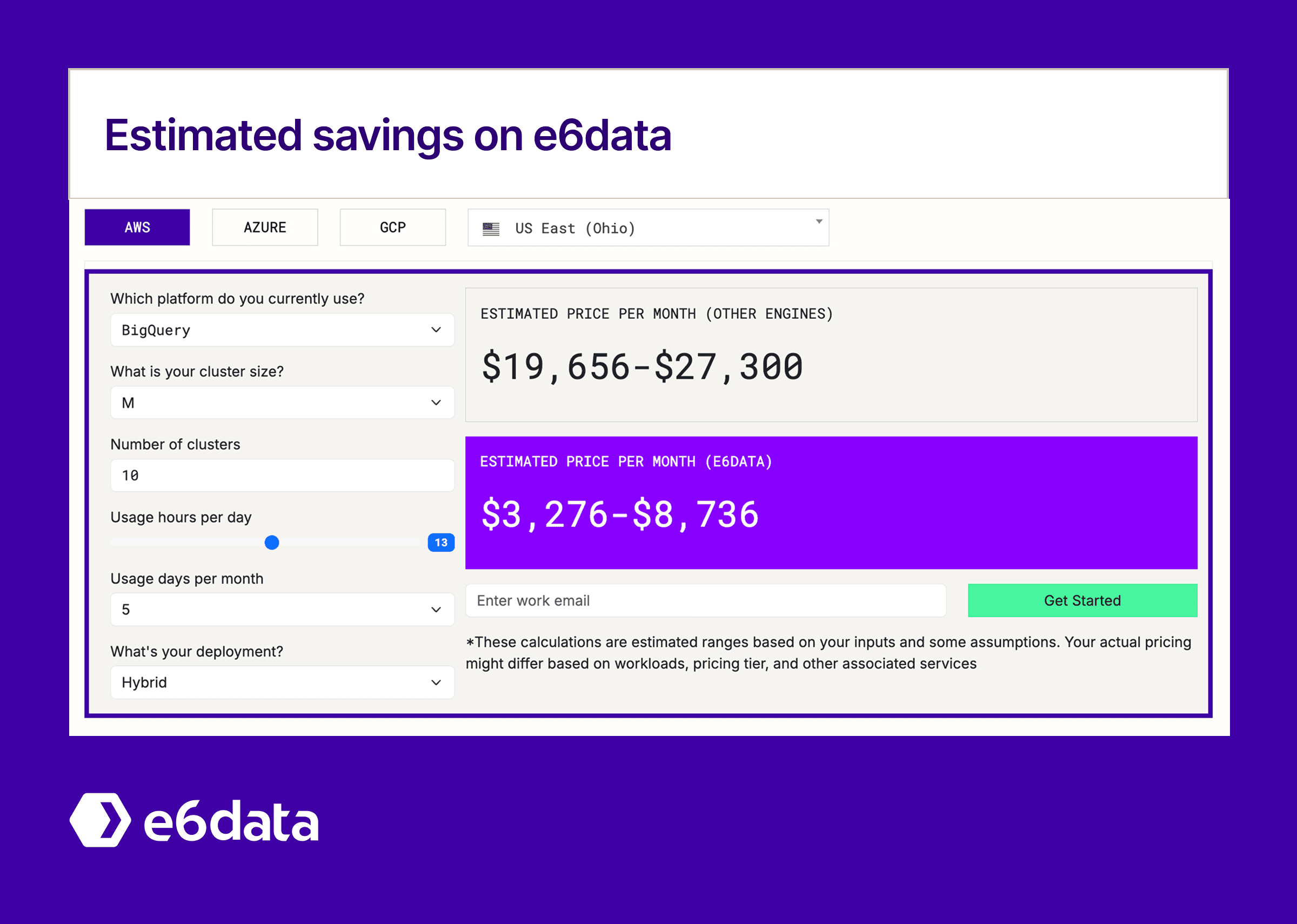
Implement BigQuery optimization tactics to capture immediate substantial cost savings, then evaluate e6data for variable analytical workloads where per-vCPU billing and automated optimization provide additional cost reductions. Leading data teams use this hybrid approach to maximize both performance and cost efficiency across their entire analytical stack.
➡️ Interested in exploring this? Start a free trial of e6data and see how it compares on your own workloads.
